Synopsis

The PLANET method has been recently proposed to quantify the relaxation parameters T₁ and T₂, the banding free magnitude, the local off-resonance ∆f₀, and the RF phase from RF phase-cycled balanced steady-state free precession (bSSFP) data. The PLANET model requires a static B₀ field over the course of the acquisition. However, due to gradient activity, B₀ drift can happen. In this work we present a study of the influence of B₀ drift on the performance of the method and we propose a strategy for correction.

Purpose

Methods

The complex phase-cycled bSSFP signal without drift can be represented as [2,3]:

$$$I = M_{eff}\frac{1-ae^{i(2πTRΔf_{0}+Δ\theta)}}{1-b\cos(2πTRΔf_{0}+Δ\theta)}e^{i(2πTEΔf_{0}+φ_{RF})} $$$ [1]

where M_eff, a, b depend on T₁, T₂, TR, FA. ∆θ is the user-controlled RF phase increment, Δf₀ is the local off-resonance, φ_RF is the combined RF transmit and receive phase.

With frequency drift modeled as Δf₀ → Δf₀ + Δf_drift(t), Eq. [1] becomes:

$$$ I = M_{eff}\frac{1-ae^{i(2πTRΔf_{0}+Δ\theta+2πTRΔf_{drift})}}{1-b\cos(2πTRΔf_{0}+Δ\theta+2πTRΔf_{drift})}e^{i(2πTEΔf_{0}+φ_{RF})}e^{i2πTEΔf_{drift}} $$$ [2]

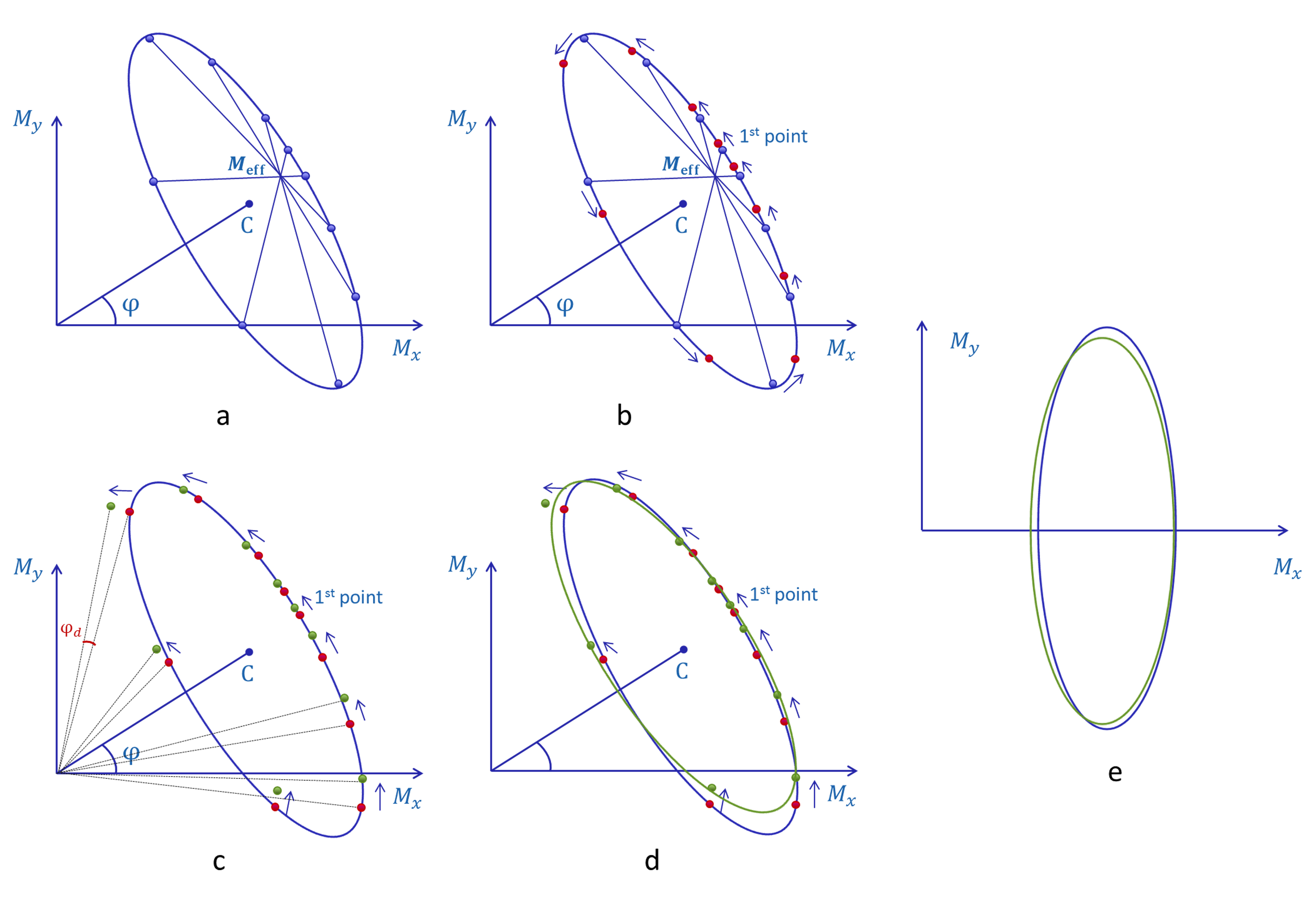
The first part of Eq.[2] multiplied by the first exponential represents the same elliptical equation as Eq.[1] with only an offset in the RF phase increment: Δθ_new = Δθ +2πTRΔf_drift. This corresponds to a drift-dependent displacement of all data points along the ellipse, see Figure 1(b). The second exponential corresponds to an additional drift-dependent rotation of all data points around the origin, see Figure 1(c,d). Ignoring the presence of drift, fitting an ellipse to the ”drifted” data points leads to a different fit compared to the fit for the “non-drifted” case, see Figure (e). After performing PLANET post-processing, this would result in errors in the parameter estimates.

We propose a 3-step correction algorithm:

1. Calculation of the spatial time-dependent B₀ drift during PLANET acquisition Δf_{drift n} (i,j)(t), where n – is the number of dynamic acquisition, t - is the time, corresponding to n^th acquisition. Assuming temporally linear drift, the frequency drift over n^th phase-cycled acquisition is estimated by:

$$$Δf_{drift,n} (i,j)(t)=n\frac{Δf_{total, drift}(i,j)}{N_{cycles}} $$$ (Hz), n = {1, ...N_cycles} [3]

where total drift over PLANET acquisition Δf_{total drift} (i,j) is calculated by subtracting two reference B₀ maps acquired right before and after PLANET acquisition.

2. Correction of M_eff, T₁, T₂ by multiplying the experimental complex data by e^{-i2πTEΔf_{drift n} (i,j)(t)}, the geometrical equivalent of which is the rotation of the “drifted” data points around the origin back to the “non-drifted” ellipse.

3. Correction of ∆f₀ and φ_RF by defining Δθ_new (i,j)(t) = Δθ(t)+2πTRΔf_drift (i,j)(t), which geometrically moves the “drifted” data points along the ellipse back to their “non-drifted” positions. Δθ(t)– is the user controlled RF phase increment.

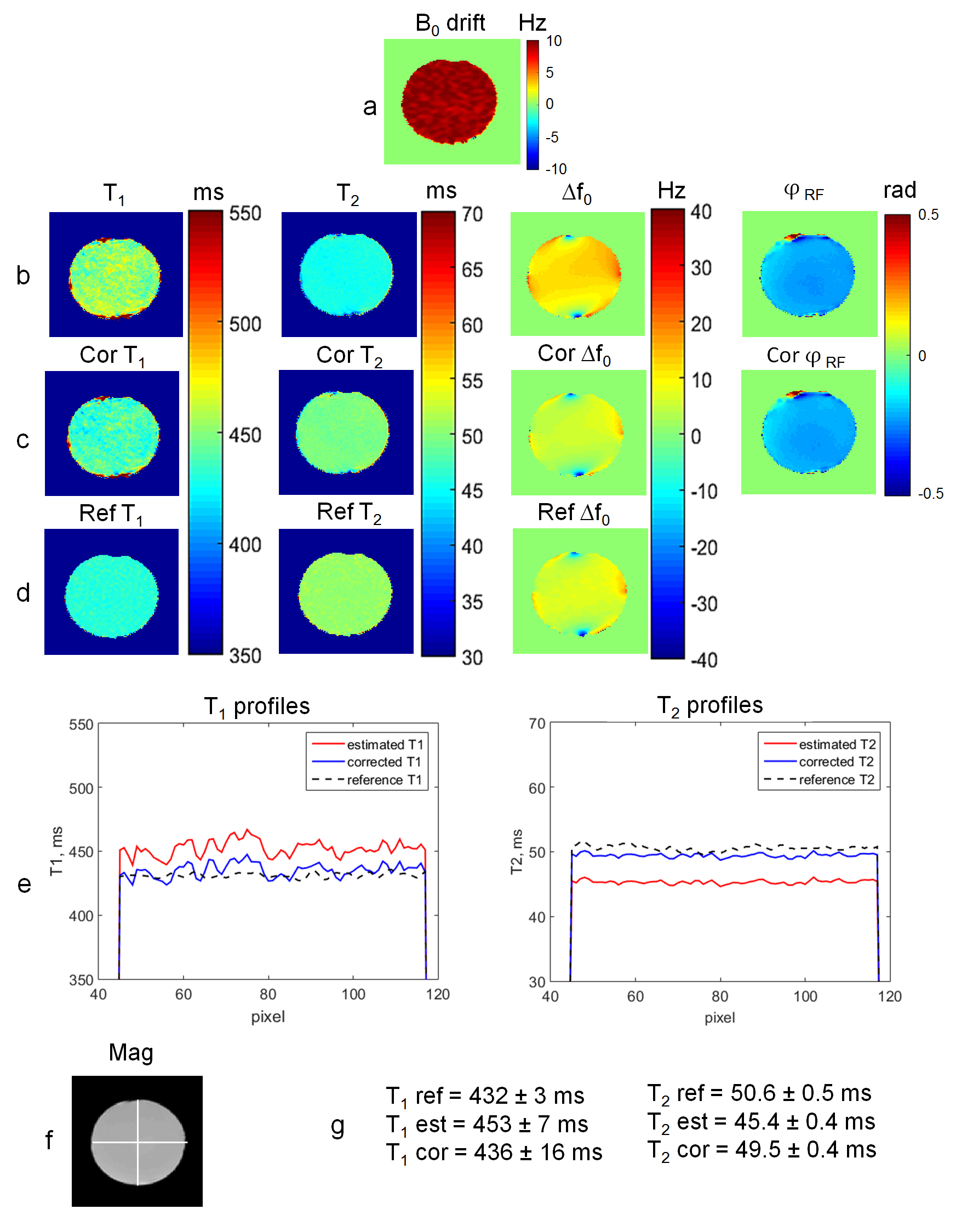
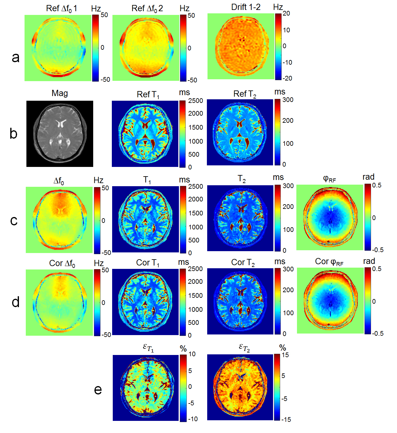
To test the correction algorithm, MRI experiments on a phantom (bottle filled with aqueous solution of MnCl₂·4H₂O) and in the brain of healthy volunteer were performed on a clinical 1.5T MR scanner (Philips Ingenia, Best, The Netherlands). A 16-channel head receive coil was used. Sequence parameter settings for 3D bSSFP: FOV 160x160x159 mm³ (phantom), 220x220x100 mm³ (the brain) , voxel size 1.1x1.1x3 mm³ (phantom), 0.98x0.98x4 mm³ (brain), TR 10 ms, FA 30˚, 10 phase cycles with Δθ = π/5. Reference B₀ maps were calculated using a dual echo approach. Reference B₁ maps were acquired for FA correction. Reference T₁ and T₂ maps were calculated using 2D MIXED method [4].

Results

Discussion and conclusion

Acknowledgements

References