4597
Wall-bounded Divergence-free Smoothing for Denoising of Velocity Data Measured by 4D Flow MRI1Dept. of Mechanical Engineering, Hanyang University, Seoul, Korea, Republic of, 2Institute of Nano Science and Technology, Hanyang University, Seoul, Korea, Republic of, 3Bioimaging Research Team, Korea Basic Science Institute, Cheongju, Korea, Republic of, 4Thoracic and Cardio-vascular Surgery, Veterans Health Service Medical Center, Seoul, Korea, Republic of, 5Neurosurgery, SMG-SNU Boramae Medical Center, Seoul, Korea, Republic of
Synopsis
Flow data measured by 4D flow MRI often result in inaccurate wall shear stress estimation due to near-wall noise in velocity measurements. We propose wall-bounded divergence-free smoothing (WB-DFS) to denoise the flow data. This method minimizes a residual error under the divergence-free condition for a wall-bounded flow and simultaneously performs data smoothing. The denoising performance of WB-DFS was found to be the best among methods reported in
INTRODUCTION
In 4D Flow MRI, accurate velocity measurements are difficult near the wall due to low signal-to-noise ratio, the partial volume effects, etc. 1-3 Therefore, a post-processing method is frequently utilized to denoise a velocity field obtained by not only 4D flow MRI measurement but other flow visualization techniques like particle image velocimetry. Recently, Wang et al. 4 proposed a divergence-free smoothing method (DFS) to minimize the residual error under a divergence-free (i.e. mass conservation) condition. Despite the superiority of this method, it is limited to be applied to an unbounded flow. Thus, we modified DFS so that it could be utilized for a wall-bounded flow like a blood vessel flow. To verify and validate the performance of WB-DFS, we compared the results of WB-DFS and other denoising techniques by applying them to noisy computational fluid dynamics (CFD) data. Then, WB-DFS is applied to a carotid artery phantom flow subject to a pulsatile flow measured by 4D flow MRI, to confirm its denoising performance and the improvement of flow visibility.METHODS
The DFS method proposed by Wang et al. 4 is based on the combination of a penalized least squares technique and the divergence corrective scheme method. Mathematically, a solution is obtained when the objective function (Eq.1) is minimized while the constraint condition (Eq.2) is satisfied.
$$ F(U_c)=(U_c-U_{exp})^T(U_c-U_{exp})+sR(U_c) \tag{1}$$
$$ subject. to. \nabla \cdot U_c = 0 \tag{2}$$
To incorporate wall-boundary information into the DFS method, the segmentation mask of a flow geometry is applied into Eq. 1 and Eq. 2, and the final solution $$$U_c$$$ can be obtained by linear algebraic calculation as follows.
$$ U_c = \Phi_{wb}(I + s\Sigma)^{-1} \Phi_{wb}^TU_{exp} \tag{3}$$
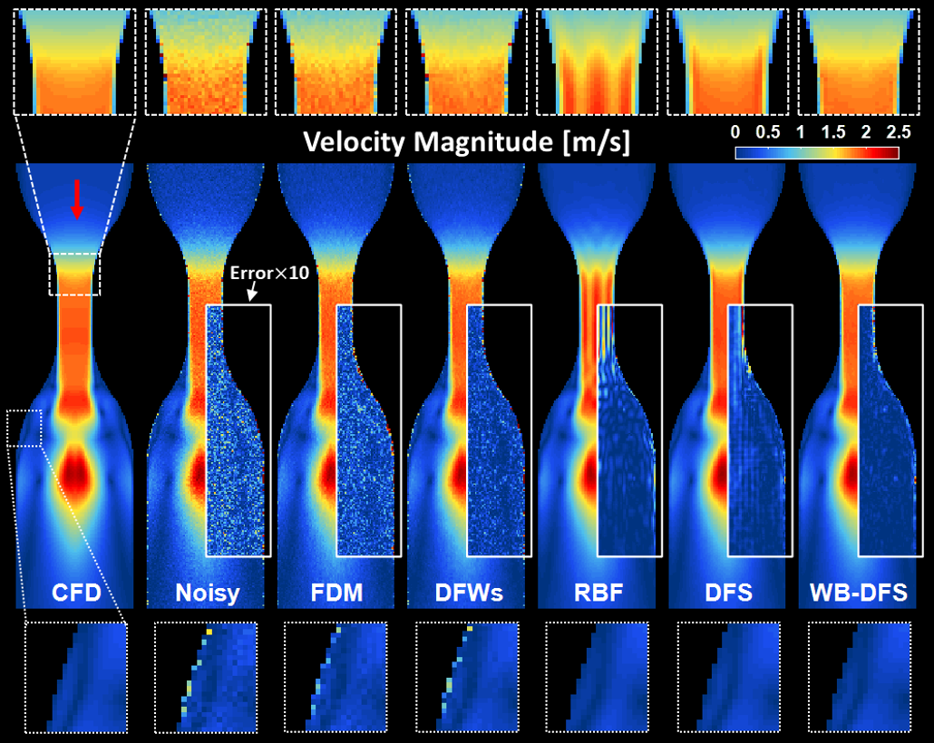
The subscript $$$c$$$ and $$$exp$$$ denote the corrected data and raw experimental data, respectively. Also, $$$\Phi_{wb}$$$, $$$\Sigma$$$, and $$$s$$$ denote the bases of WB-DFS, singular value matrix, and the smoothing parameter. To compare the denoising performance of WB-DFS and other divergence reduction methods (FDM 5, DFWs 5, RBF 6, and DFS), we used the CFD results for a stenosed pipe flow by Ong 5 as a control, and the CFD results to which 10 % Gaussian noise and near-wall outliers were added to mimic experimental data with uncertainty.
RESULTS
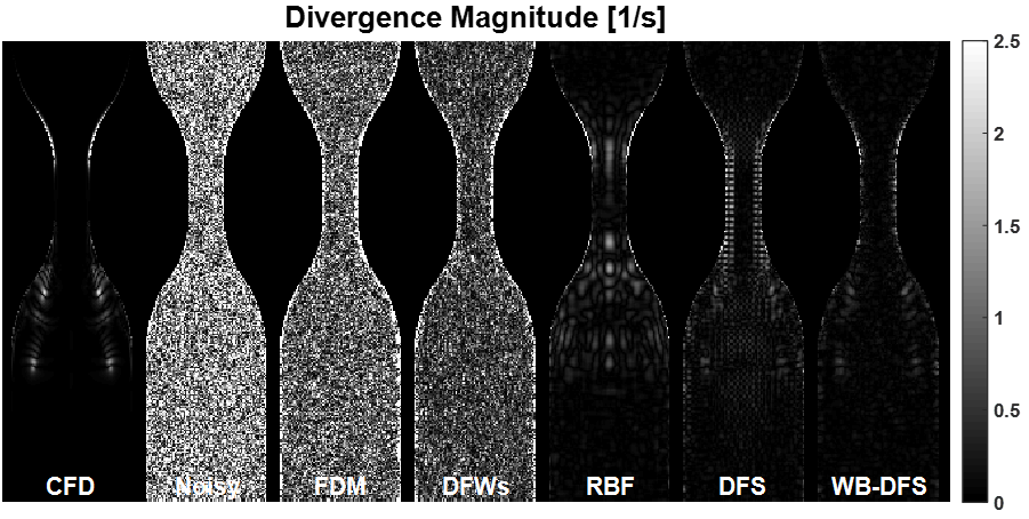
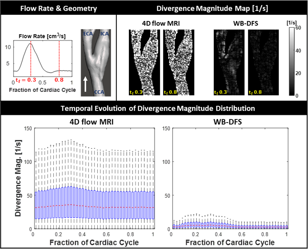
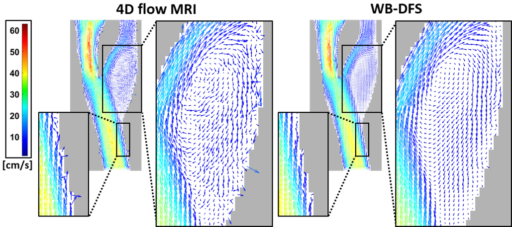
Figure 1 shows the comparison of the results of the five denoising methods applied to the noisy CFD data. WB-DFS showed a velocity magnitude distribution similar to the clean CFD results, and the velocity error is almost zero in the entire field. For example, WB-DFS shows the best performance that the divergence reduction rate was as high as 95.6% for the entire flow field and 97.6% for the near-wall regions (Figure 2). As for the carotid artery phantom measurements, WB-DFS exhibits the divergence magnitude (i.e. mass conservation error) decreased by 91% during the entire pulsatile period except the systole peak (Figure 3). As a result, a complicated flow structure such as recirculation motions in the ICA bulb after carotid endarterectomy is vividly observed without outliers so that the center of the recirculation could be determined visually (Figure 4).DISCUSSION
We developed a denoising method of WB-DFS applicable to a wall-bounded flow and it showed a superior divergence reduction performance, especially near wall. Clinically important hemodynamic parameters like wall shear stress (WSS) and oscillatory shear index (OSI) are obtained by differentiating the near-wall velocities that contain a relatively high level of noise due to a low SNR of 4D flow MRI. Thus, the essence of this study lies in that it can improve the accuracy of WSS or OSI estimation for a given data of flow imaging and the reliability of hemodynamic diagnosis of cardiovascular diseases. Additionally, WB-DFS does not require a user to determine any denoising parameters included in Eq.1 through 3 because it automatically and mathematically determines the optimal solution for a given geometry shape and flow field using a generalized cross validation function. 7CONCLUSION
A divergence-free smoothing method applicable to wall-bounded flow has been developed for denoising velocity data obtained by 4D flow MRI. The results indicate that it preserves the essential characteristics of the raw velocity data while reducing erroneous velocity vectors for a stenosed pipe flow generated by CFD and carotid artery phantom flow measured by 4D flow MRI. WB-DFS is expected to improve the estimation accuracy of WSS or OSI required for the reliable diagnosis of cardiovascular diseases.Acknowledgements
This work was supported by the National Research Foundation of Korea (NRF) grant funded by the Korea government (No. 2016R1A2B3009541 and 2012R1A6A1029029).References
- Nayak KS, Nielsen J-F, Bernstein MA, et al. Cardiovascular magnetic resonance phase contrast imaging. Journal of Cardiovascular Magnetic Resonance 2015;17(1):71.
- Lustig M, Pauly JM. SPIRiT: Iterative self‐consistent parallel imaging reconstruction from arbitrary k‐space. Magnetic resonance in medicine 2010;64(2):457-471.
- Markl M, Bammer R, Alley M, et al. Generalized reconstruction of phase contrast MRI: analysis and correction of the effect of gradient field distortions. Magnetic resonance in medicine 2003;50(4):791-801.
- Wang C, Gao Q, Wang H, Wei R, Li T, Wang J. Divergence-free smoothing for volumetric PIV data. Experiments in Fluids 2016;57(1):15.
- Ong F, Uecker M, Tariq U, et al. Robust 4D flow denoising using divergence‐free wavelet transform. Magnetic resonance in medicine 2015;73(2):828-842.
- Busch J, Giese D, Wissmann L, Kozerke S. Reconstruction of divergence‐free velocity fields from cine 3D phase‐contrast flow measurements. Magnetic resonance in medicine 2013;69(1):200-210.
- Craven P, Wahba G. Smoothing noisy data with spline functions. Numerische mathematik 1978;31(4):377-403.
Figures