4596

Artifact correction in spiral trajectory with high gradient performance

Daehun Kang¹, Uten Yarach¹, Joshua D Trzasko¹, Myung-Ho In¹, Erin M Gray¹, Ek Tsoon Tan², Nolan K Meyer¹, Thomas K Foo², Yunhong Shu¹, John Huston¹, and Matt A Bernstein¹

¹Department of Radiology, Mayo Clinic, Rochester, MN, United States, ²GE Global Research, Niskayuna, NY, United States

Synopsis

A low-cryogen, compact 3T MRI is equipped with high performance gradients, of which increased maximum gradient amplitude and slew rate can improve MR image quality of spiral trajectory to reduce susceptibility and off-resonance effect. However, use of the higher slew rate and gradient strength with an Archimedean spiral trajectory can lead to rotation artifacts and a local blurring. In this work, we corrected those artifacts with using a dynamic field camera and with attention to the azimuthal Nyquist sampling criterion.

Introduction

Increased maximum gradient amplitude and slew rate can improve MR image quality for echo planar imaging (EPI) by reducing echo spacing.¹ A low-cryogen, compact 3T MRI equipped with a high-performance gradient system producing maximum amplitude of 80 mT/m with a slew rate of 700 T/m/s has been reported.^2-7 Similar to EPI, spiral trajectories benefit from high performance gradients by reducing the readout duration, and consequently reducing susceptibility and other off-resonance effects.⁸ However, utilizing the higher slew rate and gradient strength with a spiral trajectory can lead to severe rotation artifacts and image blurring, which are distinct from off-resonance effects. In this work, we used a dynamic field camera to measure the true trajectories and applied them to correct the artifacts. The receiver bandwidth requirement was also considered to eliminate under-sampling artifacts when high slew rates were used.

Methods

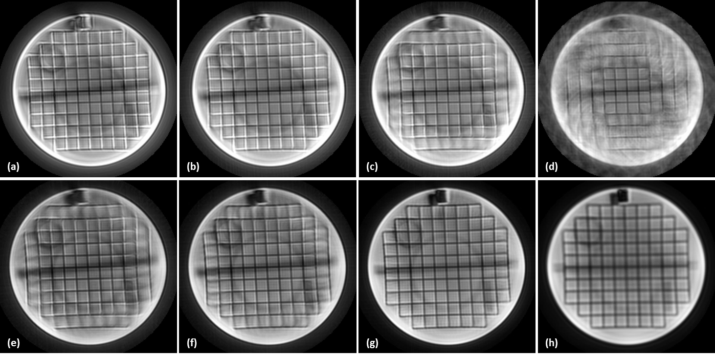
Azimuthal Nyquist sampling criterion. While radial Nyquist sampling is regularly considered in a mathematical procedure for designing a spiral trajectory,⁹ azimuthal Nyquist sampling only becomes an issue with high amplitude gradients, which cause the rapid traversal of k-space to outpace the sampling rate. Consider the equation: $$$\frac{\gamma}{2\pi}G_{max}\cdot{FOV}=2\Delta\nu$$$,¹⁰ where $$$\pm\Delta\nu$$$ and $$$G_{max}$$$ are the receiver bandwidth and maximum gradient amplitude for spiral trajectory, respectively. To investigate azimuthal aliasing, data was obtained with various $$$\Delta\nu$$$ or maximum slew rates ($$$S_{max}$$$). Also, the transient times to reach $$$G_{max}$$$ were investigated depending on $$$S_{max}$$$.

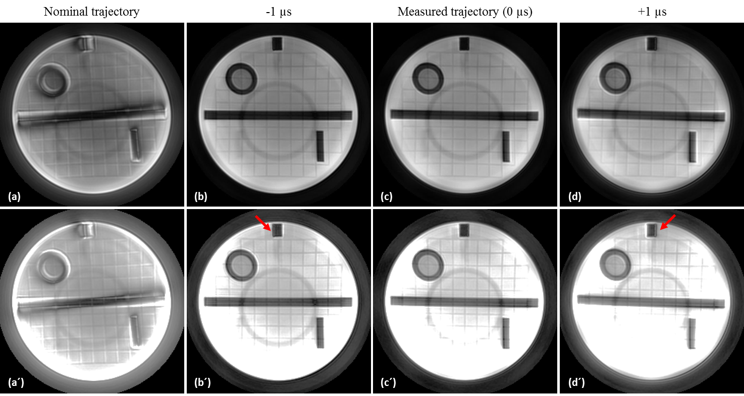
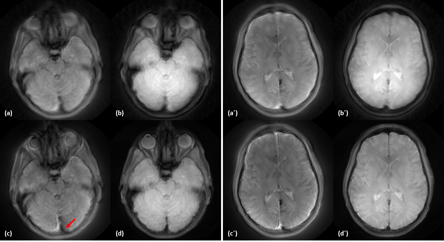
Spiral trajectory measured by dynamic field camera. The eddy current and the system delay cause the mismatch between designed and actual spiral trajectories.¹¹ A dynamic field camera with NMR field probes containing ¹⁹F (Skope,Zurich,Switzerland)^12,13 was utilized to obtain 1^st-order k-space terms of k_x & k_y at 1.0 MHz sampling rate with the American College of Radiology (ACR) MRI phantom.¹⁴ The dynamic field was repeatedly acquired for 4.4 ms to include the measurement of each interleave (e.g., “arm”) of the spirals. k_x & k_y were resampled by $$$\frac{1}{2\Delta\nu}$$$ sec. to determine actual trajectories, and the timing to start trajectories was selected by adjusting 1 µs to maximally enhance an image quality of the phantom. The same trajectories were applied to the reconstruction of human subject data (acquired under an IRB-approved protocol and following written informed consent).

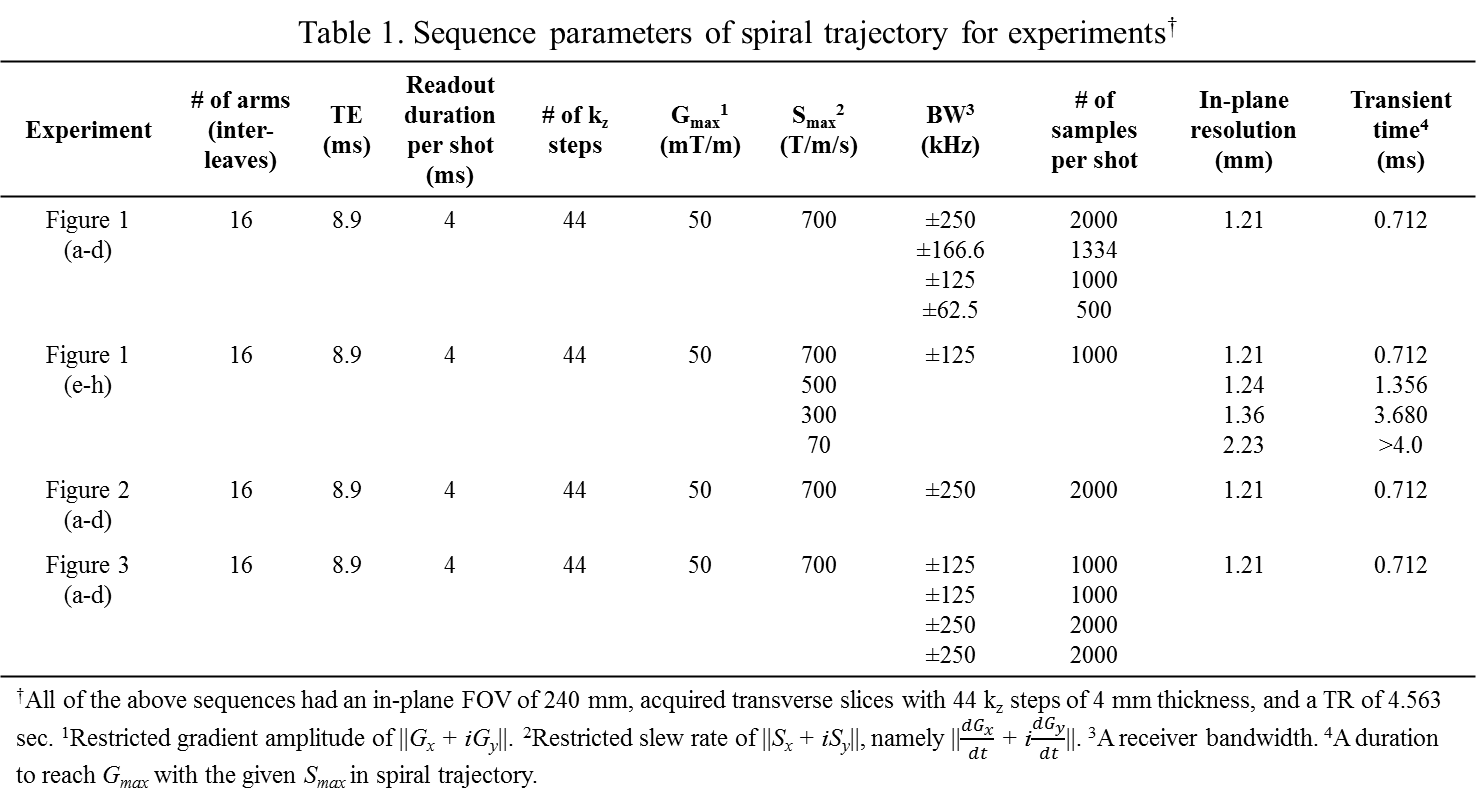
Sequence parameters. The 3D fast spin-echo stack of spirals¹⁵ was used with imaging parameters in Table 1, which is for pCASL sequence. Image reconstruction via density compensated gridding was performed with Orchestra (GE Healthcare,Waukesha,WI,US) in Matlab (The MathWorks,Inc.,Natick,MA,US).

Results

Since the azimuthal Nyquist sampling criterion suggests that $$$\Delta\nu$$$ of ±255.4 kHz is sufficient in the case of FOV=240 mm and $$$G_{max}$$$=50 mT/m, the image acquired with $$$\Delta\nu$$$ of ±250 kHz shows little azimuthal aliasing in Fig.1. Also, the aliasing artifact seems to be mitigated by a low $$$S_{max}$$$ even with $$$\Delta\nu$$$ of ±125 kHz.

Figure 2 shows images reconstructed with nominal and measured trajectories. A nominal trajectory with $$$S_{max}$$$=700 T/m/s demonstrated reduced image quality and counterclockwise image rotation. Additionally, the image with the optimal trajectory was compared with those with other trajectories of different timings. This demonstrates that precise matching between an acquired data and a resampled trajectory is required. In Fig.3, the artifact correction with the optimal trajectory used previously was applied on volunteer data.

Discussion

In this work, the artifacts generated by high $$$S_{max}$$$ in a given $$$G_{max}$$$ were investigated in spiral imaging. We showed that artifacts can be caused by two different types of sources, namely, azimuthal aliasing and gradient delay causing the designed and actual spiral trajectories to differ.

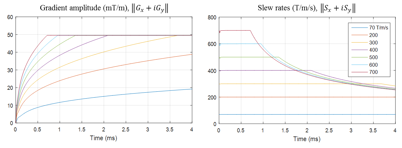
Higher $$$S_{max}$$$ produces a shorter transient time and results in the efficient use of gradient strength in spiral imaging. For example in Fig.4, although $$$S_{max}$$$ below 200 T/m/s could not reach $$$G_{max}$$$ within 4 ms, $$$S_{max}$$$ of 700 T/m/s produces only 0.712 ms in transient time and then $$$G_{max}$$$ was applied to 82.2% of acquired k-space data. Therefore, with high $$$S_{max}$$$, it is important to consider the appropriate selection of sampling bandwidth.

A dynamic field camera provided data to correct the gradient deviation artifact. Notably, the same measured data that was used to correct the spiral trajectory was successfully applied to data obtained from a human volunteer. This suggests that the error in k_x & k_y is system-specific rather than object-specific. A further study is required with higher-order terms. Finally, the trajectory obtained by a dynamic field camera is expected to be useful for applications that use low slew rates or a low spatial resolution, such as ASL.¹⁶

Conclusion

The maximum slew rate of 700T/m/s with Archimedean spiral trajectory results in artifacts with spiral imaging. These were corrected by a trajectory measured with a dynamic field camera, and by providing attention to the azimuthal Nyquist sampling criterion.

Acknowledgements

The authors would like to thank Eric W Fiveland from GE Global Research for his help in supporting use of Skope system. This work was supported in part by research grant NIH U01-EB024450.

References

1 Tan, E. T. et al. High slew-rate head-only gradient for improving distortion in echo planar imaging: Preliminary experience. J Magn Reson Imaging 44, 653-664, doi:10.1002/jmri.25210 (2016).

2 Lee, S. K. et al. Peripheral nerve stimulation characteristics of an asymmetric head-only gradient coil compatible with a high-channel-count receiver array. Magn Reson Med 76, 1939-1950, doi:10.1002/mrm.26044 (2016).

3 Foo, T. K. F. et al. Lightweight, compact, and high-performance 3T MR system for imaging the brain and extremities. Magn Reson Med 80, 2232-2245, doi:10.1002/mrm.27175 (2018).

4 Weavers, P. T. et al. Technical Note: Compact three-tesla magnetic resonance imager with high-performance gradients passes ACR image quality and acoustic noise tests. Med Phys 43, 1259-1264, doi:10.1118/1.4941362 (2016).

5 Weavers, P. T. et al. B0 concomitant field compensation for MRI systems employing asymmetric transverse gradient coils. Magn Reson Med 79, 1538-1544, doi:10.1002/mrm.26790 (2018).

6 Tao, S. et al. Gradient nonlinearity calibration and correction for a compact, asymmetric magnetic resonance imaging gradient system. Phys Med Biol 62, N18-N31, doi:10.1088/1361-6560/aa524f (2017).

7 Tao, S. et al. Gradient pre-emphasis to counteract first-order concomitant fields on asymmetric MRI gradient systems. Magn Reson Med 77, 2250-2262, doi:10.1002/mrm.26315 (2017).

8 Tao, S. et al. in Proc. Intl. Soc. Mag. Reson. Med. #0936 (2018).

9 King, K. F., K. F. Foo, T. & Crawford, C. R. Optimized gradient waveforms for spiral scanning. Magn Reson Med, doi:10.1002/mrm.1910340205 (1995).

10 Bernstein, M. A., King, K. F. & Zhou, X. J. Handbook of MRI Pulse Sequence, Ch. Spiral, 937-940 (2004).

11 Bhavsar, P. S., Zwart, N. R. & Pipe, J. G. Fast, variable system delay correction for spiral MRI. Magn Reson Med, doi:10.1002/mrm.24730 (2014).

12 Kasper, L. et al. Rapid anatomical brain imaging using spiral acquisition and an expanded signal model. NeuroImage, doi:10.1016/j.neuroimage.2017.07.062 (2018).

13 Dietrich, B. E. et al. A field camera for MR sequence monitoring and system analysis. Magn Reson Med 75, 1831-1840, doi:10.1002/mrm.25770 (2016).

14 Phantom test guidance for the ACR MRI accreditation program. The American College of Radiology. (Reston, Virginia, 2000).

15 Ye, F. Q., Frank, J. A., Weinberger, D. R. & McLaughlin, A. C. Noise reduction in 3D perfusion imaging by attenuating the static signal in arterial spin tagging (ASSIST). Magn Reson Med 44, 92-100 (2000).

16 Alsop, D. C. et al. Recommended implementation of arterial spin-labeled perfusion MRI for clinical applications: A consensus of the ISMRM perfusion study group and the European consortium for ASL in dementia. Magn Reson Med 73, 102-116, doi:10.1002/mrm.25197 (2015).

Figures

Figure 1. Effect of azimuthal aliasing depending on a receiver bandwidth or a maximum slew rate. The image blurring occurred perpendicular to a radial direction from the border of an image. The images were obtained with various receiver bandwidths of (a) ±250, (b) ±166.6, (c) ±125 and (d) ±62.5 kHz with a slew rate of 700 T/m/s and with various slew rates of (e) 700, (f) 500, (g) 300 and (h) 70 T/m/s with a receiver bandwidth of ±125 kHz. Even when ∆v is lower than that criterion, the artifact seems to be mitigated with a low maximum slew rate like (g,h).

Figure 2. Effects of spiral trajectory measured by dynamic field camera. (a) The image was reconstructed by the spiral trajectory designed with a maximum slew rate of 700T/m/s and a maximum gradient amplitude of 50mT/m. The measured trajectory was determined by resampling waveforms of the 1st-order terms (k_x & k_y) monitored by a dynamic field camera with a sampling interval of 2µs. (c) The image from the determined trajectory was compared with those from the candidate trajectories (b) leading to and (d) lagging by 1µs. (a´-d´) The same images having different brightness with (a-d), respectively, were plotted to show differences as indicated by red arrows.

Figure 3. Proton-density-weighted images of a human volunteer. In a top-down direction of (a)-to-(c) and (b)-to-(d), the local blurring on the image was significantly reduced by applying an appropriate bandwidth of ±250 kHz instead of ±125 kHz. The left-to-right direction of (a)-to-(b) and (c)-to-(d) shows the effect of the correction for spiral trajectory. In the procedure of (c) to (d), the measured trajectories same with those in Figure 2 was applied to data from a volunteer and consequently the artifact of an image rotation (red arrow) was solved. (a´-d´) A slice on a different location was plotted with the same organization with (a-d).

Figure 4. Evolution of gradient amplitudes and slew rates over 4 ms, depending on $$$S_{max}$$$ in a fixed $$$G_{max}$$$ of 50 mT/m. The larger $$$S_{max}$$$ produces the shorter transient time.

Table 1

Proc. Intl. Soc. Mag. Reson. Med. 27 (2019)

4596