4574
Capturing Time-Dependent Electric Currents Using MRI with A Sub-Millisecond Temporal Resolution1Center for MR Research, University of Illinois at Chicago, Chicago, IL, United States, 2Bioengineering, University of Illinois at Chicago, Chicago, IL, United States, 3Radiology, University of Illinois at Chicago, Chicago, IL, United States, 4Neurosurgery, University of Illinois at Chicago, Chicago, IL, United States
Synopsis
Neuronal current mapping using MRI has profound biomedical applications, but is hampered by limited temporal resolution. Using a technique known as Sub-Millisecond Imaging of cycLic Event or SMILE, we demonstrate that the temporal resolution of MRI can be substantially increased to the sub-millisecond scale or shorter. This allows capturing ultra-fast physical or biological processes that are cyclic. Although our experimental studies are limited to mapping time-varying currents in a phantom, the same concept can be extended to capturing more complex biological processes, including but not limited to, neuronal currents.
Introduction
Mapping time-dependent electric currents using MRI was proposed three decades ago1, and has since stimulated considerable interest in capturing neuronal activation associated with brain functions2. This possibility, however, faces two daunting challenges – a very weak current (nano-ampere) and an ultrafast temporal scale (millisecond) during neuronal activities. Although considerable progresses have been made in addressing the first problem3,4, the challenge of temporal resolution remains formidable. Even with the most advanced k-space traversal strategies, image reconstruction algorithms5–8, and RF coil technologies9, the achievable temporal resolution of MRI (i.e., tens of millisecond) reported to date falls short for capturing the rapid current change during neuronal activation. We herein demonstrate an MRI technique – Sub-Millisecond Imaging of cycLic Event or SMILE – that is capable of capturing cyclic electric current changes with a sub-millisecond temporal resolution, to illustrate a technical possibility towards mapping neuronal currents and other ultrafast biological processes.Materials and Methods
SMILE:
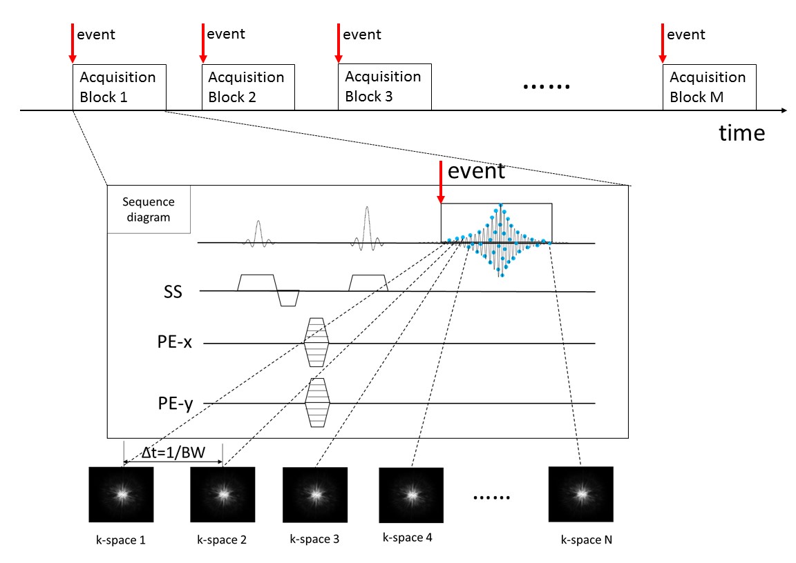
Unlike conventional MRI in which an FID or a spin-echo signal is used to encode spatial or chemical shift information, SMILE uses the signal to resolve a dynamic event with a temporal resolution determined by the dwell time. In SMILE, spatial localization is accomplished by phase-encoding and/or slice selection only, freeing up the conventional frequency-encoding domain for temporal characterization. Each phase-encoding step is synchronized with the periodicity of a cyclic event, and each point in the FID or spin-echo signal corresponds to an image. A collection of all points over the course of an FID or spin-echo signal provides a time-resolved characterization of the cyclic event, as shown in Fig.1. With SMILE, the temporal resolution of MRI is no longer determined by how fast k-space is traversed, but by the dwell time or the receiver bandwidth.
Apparatus:
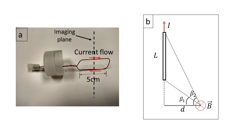
A rectangular wire loop with a length of 5cm (Fig. 2a) was constructed and submerged in a water phantom for the experimental studies. The magnetic field produced by the wire loop can be calculated using the Biot-Savart law.$$B(t)=\int_{L}^{}dB= \frac{\mu_{0}I(t)}{4\pi d}(sin\beta_2-sin\beta_1),$$ where L is the length of the wire, μ0 is the magnetic permeability, I is the current, and other geometric parameters are defined in Fig. 2b. With an applied current, a corresponding phase change in the image can be calculated as:$$\phi(t)=\gamma\int_{0}^{t} B(t^{'})dt^{'}.$$
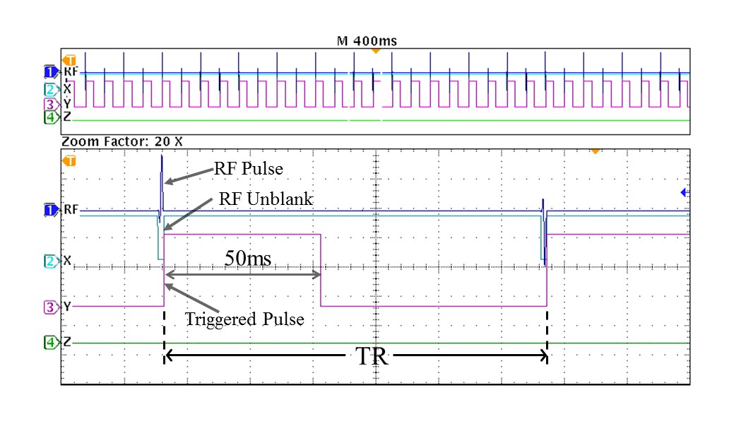
A pulse generator, PulsePal (Sanworks, Stony Brook, NY), was used to deliver a current signal to the wire loop10 in synchrony with a SMILE pulse sequence. For simplicity, a step current waveform and a sine waveform were employed in this study. The RF unblank signal from the scanner was used as a trigger for synchronization, as illustrated in Fig. 3.
Simulation:
To determine the relationship between the applied current and the phase change, a computer simulation was performed with a set of parameters identical to those used in the experimental studies described below. Using Eqs. [1] and [2], the simulated images also established a benchmark for comparison with experimental images.
Data Acquisition and Analysis:
A SMILE sequence (Fig. 1) was implemented on a 3T GE MR750 scanner, followed by experimental studies using the apparatus in Figs. 2 and 3 with the following parameters: TR=122ms, TE=2.8ms, slice thickness=3mm, FOV=8cm×8cm, matrix=64×64, bandwidth=±2.5kHz, number of sampling points=256, scan time=8:20. The acquisition was first performed without current in the wire loop as a reference, followed by another acquisition after applying a 3mA peak current with a duration of 50ms. Using Eq. [2], phase maps were produced by taking the phase difference between the two acquisitions and compared with the simulation results.
Results
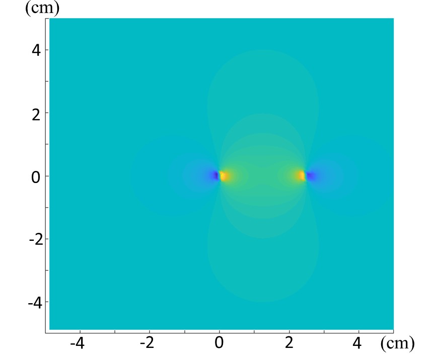
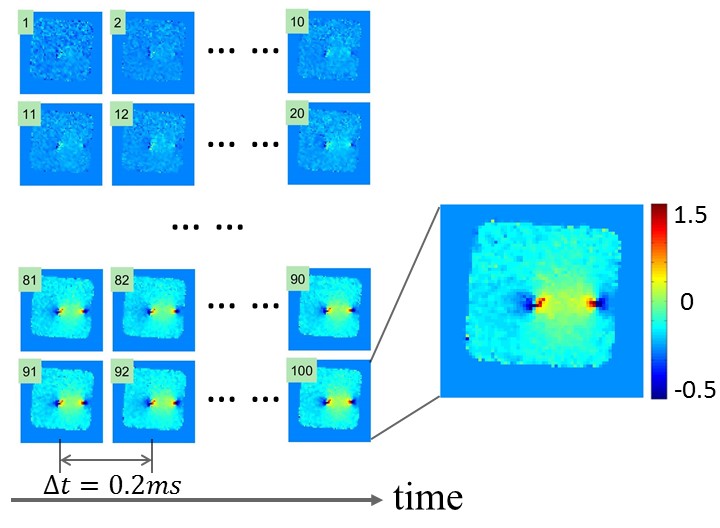
Figure 4 shows a simulated phase image at the middle plane of two parallel wires (Fig. 2a) with a current of 3mA, where the dipole pattern is clearly visible. For the experimental study, the fast-changing phase maps as a result of the step current waveform in the wire were well captured with a temporal resolution of 0.2ms, as shown in Figure 5. The results from the simulation and experiment matched well qualitatively and quantitatively. Similar results were achieved using a sine current waveform.Discussion and Conclusion
Using SMILE, we have successfully captured the rapid phase evolution caused by time-varying currents with a temporal resolution of 0.2ms. Although we have used simple current waveforms to demonstrate SMILE, the same concept can be extended to capturing more complex rapid physical and biological processes, including but not limited to, neuronal currents, provided that the process is cyclic. In addition, although the present demonstration is limited to sub-millisecond, SMILE can be extended to higher temporal resolutions with a broader receiver bandwidth.Acknowledgements
This work was supported in part by NIH 1S10RR028898.References
1. Joy, M., Scott, G. and Henkelman, M. In vivo detection of applied electric currents by magnetic resonance imaging. Magn. Reson. Imaging 7, 89–94 (1989).
2. Luo, Q., Jiang, X., Chen, B., Zhu, Y. and Gao, J.-H. Modeling neuronal current MRI signal with human neuron. Magn. Reson. Med. 65, 1680–1689 (2011).
3. Konn, D., Gowland, P. and Bowtell, R. MRI detection of weak magnetic fields due to an extended current dipole in a conducting sphere: A model for direct detection of neuronal currents in the brain. Magn. Reson. Med. 50, 40–49 (2003).
4. Xiong, J., Fox, P. T. and Gao, J.-H. Directly mapping magnetic field effects of neuronal activity by magnetic resonance imaging. Hum. Brain Mapp. 20, 41–49 (2003).
5. Pruessmann, K. P., Weiger, M., Scheidegger, M. B. and Boesiger, P. SENSE: sensitivity encoding for fast MRI. Magn. Reson. Med. 42, 952–962 (1999).
6. Griswold, M. A. Jakob, P. M., Heidemann, R.M. et al. Generalized autocalibrating partially parallel acquisitions (GRAPPA). Magn. Reson. Med. 47, 1202–1210 (2002).
7. Lustig, M., Donoho, D. and Pauly, J. M. Sparse MRI: The application of compressed sensing for rapid MR imaging. Magn. Reson. Med. 58, 1182–1195 (2007).
8. Sodickson, D. K. and Manning, W. J. Simultaneous acquisition of spatial harmonics (SMASH): Fast imaging with radiofrequency coil arrays. Magn. Reson. Med. 38, 591–603 (1997).
9. Wright, S. M. and McDougall, M. P. Single echo acquisition MRI using RF encoding. NMR Biomed. 22, 982–993 (2009).
10. Sanders, J. I. and Kepecs, A. A low-cost programmable pulse generator for physiology and behavior. Front. Neuroengineering 7, (2014).
Figures