4547
Deep parameter mapping with relaxation signal model driven constraints1Electrical and Computer Engineering, University of Arizona, Tucson, AZ, United States, 2Department of Medical Imaging, University of Arizona, Tucson, AZ, United States, 3Biomedical Engineering, University of Arizona, Tucson, AZ, United States
Synopsis
Conventional MR parameter mapping suffers from long acquisition times limiting their clinical utility. Model based iterative methods have been proposed to allow reconstructions from highly accelerated data, but these suffer from high computational costs. Deep learning based methods that can reduce reconstruction times significantly while yielding reconstruction quality comparable to the model based methods have emerged recently. In this work, we evaluate the use of signal model driven constraints in deep learning based MR parameter mapping.
Introduction
Quantitative mapping of MR parameters is becoming increasingly popular for tissue characterization and pathological assessment but suffers from long acquisition times limiting their clinical utility. Model-based compressive sensing (CS) methods1-5 have been proposed to enable high quality reconstructions from clinically acceptable scan times (high acceleration rates). However, these methods are usually associated with high computational costs. Recently, deep learning based parameter mapping methods6-9 that can dramatically improve reconstruction times while yielding comparable reconstruction quality as the CS methods have emerged. In
this work, we introduce signal model driven constraints in deep parameter
mapping and evaluate the use of these constraints at different stages of the
network. Methods
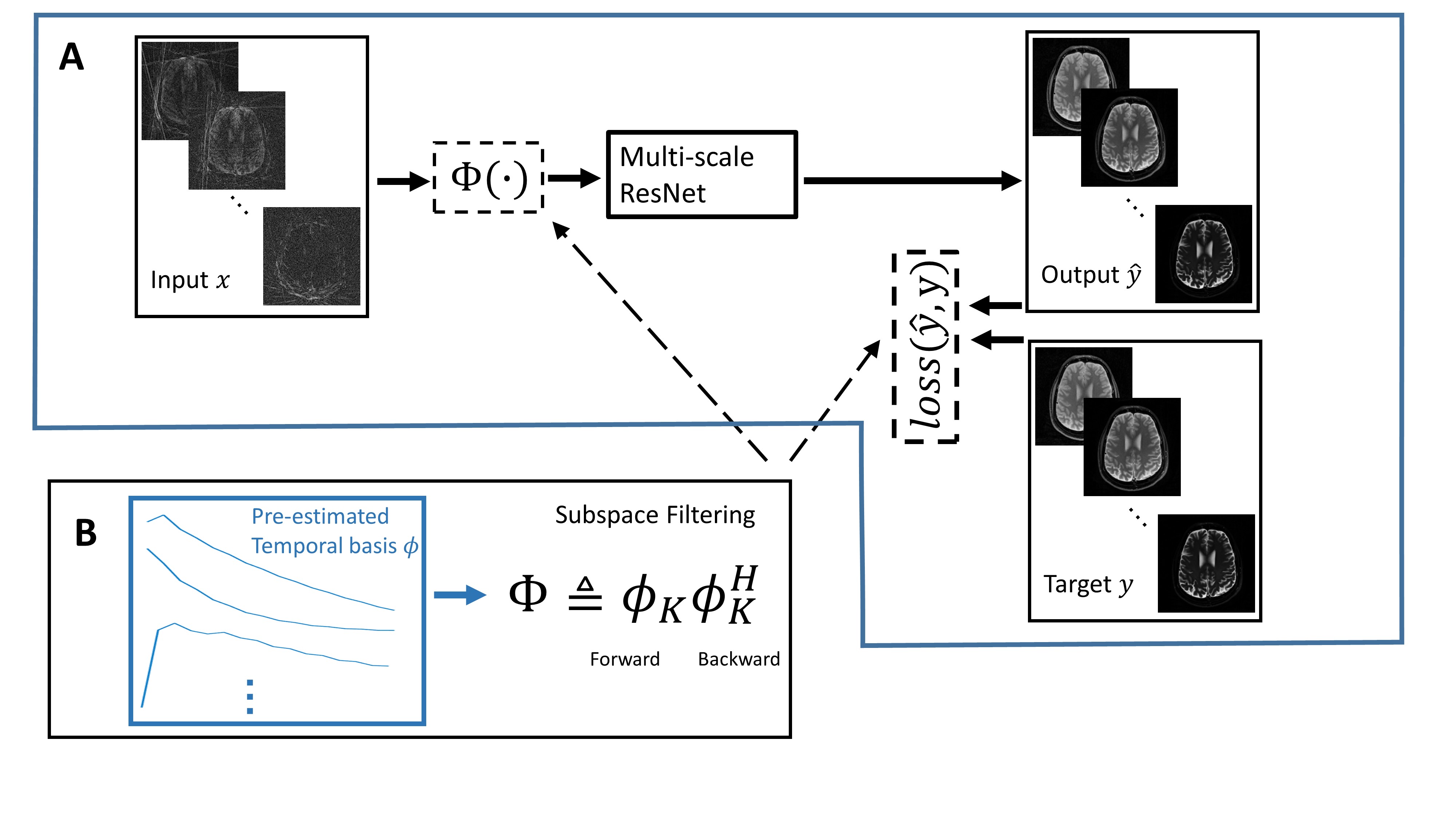
Our proposed approach (Fig. 1A) is to train a supervised network for restoring multi-contrast images from highly undersampled multi-contrast radial data. This supervised network is a multi-scale ResNet6 parameterized by weights $$$w$$$. The inputs $$$x$$$ to the network were created by applying NUFFT10 to undersampled k-space data at each contrast. The targets $$$y$$$ were obtained using a model-based CS method, NLR3D11, from the same undersampled k-space data. As pointed out in many model-based CS methods,1-5 an orthogonal basis that models the temporal characteristics of relaxation signals can be obtained via principal components analysis. We define subspace filtering as the joint forward and backward projection onto this truncated temporal basis (Figure 1B). This dimensionality reduction explicitly constrains reconstructions to a low-dimensional space and greatly reduces the undersampling artifacts and noise amplification in NUFFT reconstructions.4 This approach can be used as a preprocessing step for network training (Fig. 1A) by applying subspace filtering to all input data. Alternatively, subspace filtering can be incorporated into the network training loss. We first consider a conventional L1 loss function without subspace filtering:
$$argmin_w||y-\hat{y}(x,w)||_1 \quad (1)$$
where $$$y$$$ represents the target of network and the output $$$\hat{y}$$$ is a function of input $$$x$$$ and weights $$$w$$$. Alternatively, the principal components basis (PCB)12,13 can be incorporated into the training loss as
$$argmin_w||y-\hat{y}\phi\phi^H||_1 \quad (2)$$
Finally, instead of a hard subspace constraint, the MOdel Consistency COndition (MOCCO)4 can be incorporated into the training loss as a regularization term:
$$argmin_w||y-\hat{y}||_1+\lambda||\hat{y}-\hat{y}\phi\phi^H||_1 \quad (3)$$
For axial brain T1 mapping, undersampled data (R=32) were acquired from 6 volunteers using an Inversion Recovery radial SSFP (IR-radSSFP) sequence14 with sequence parameters TR=4.92ms, TE=2.4ms, 32 TIs, resolution=0.69mm x 0.69mm, slice thickness=3mm, 40 slices, and 16 lines/TI with 320 readout points/line. For axial abdomen T1 mapping, undersampled data (R=38) were acquired from 9 volunteers using IR-radSSFP sequences with sequence parameters TR=4.40ms, TE=2.15ms, 32 TIs, resolution=0.8mm x 0.8mm, slice thickness=3mm, 10 slices, and 16 lines/TI with 384 readout points/line. Data augmentation and training procedures described in6 were followed for all multi-scale ResNets using 64x64 patches. One subject was randomly selected for validation and another subject for testing. The remaining subjects were used for training. All networks were implemented in PyTorch15 using ADAM optimizer for training with a learning rate of 1e-4. λ=0.01 was selected in the MOCCO loss. The complex-valued data were split into real and imaginary part before they are fed to the networks. Bloch simulations were used to generate training signal curves for T1 experiments and the corresponding subspace bases were obtained using PCA. Four PCs were used for all the experiments.
Results
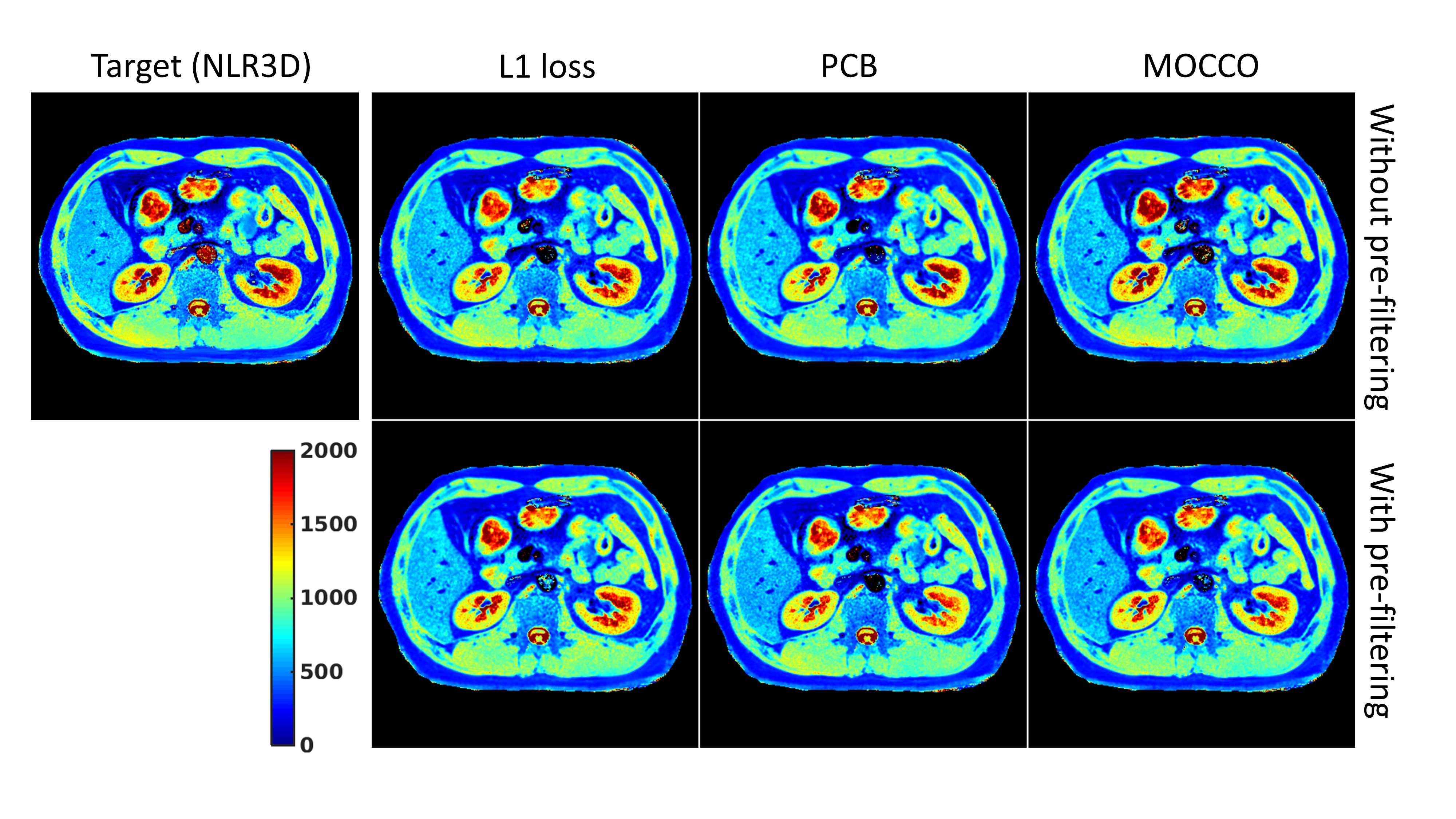
Fig.2
shows the abdominal T1 mapping results using L1, PCB, MOCCO losses with and without
pre-subspace filtering. All networks were able to converge during training and produced
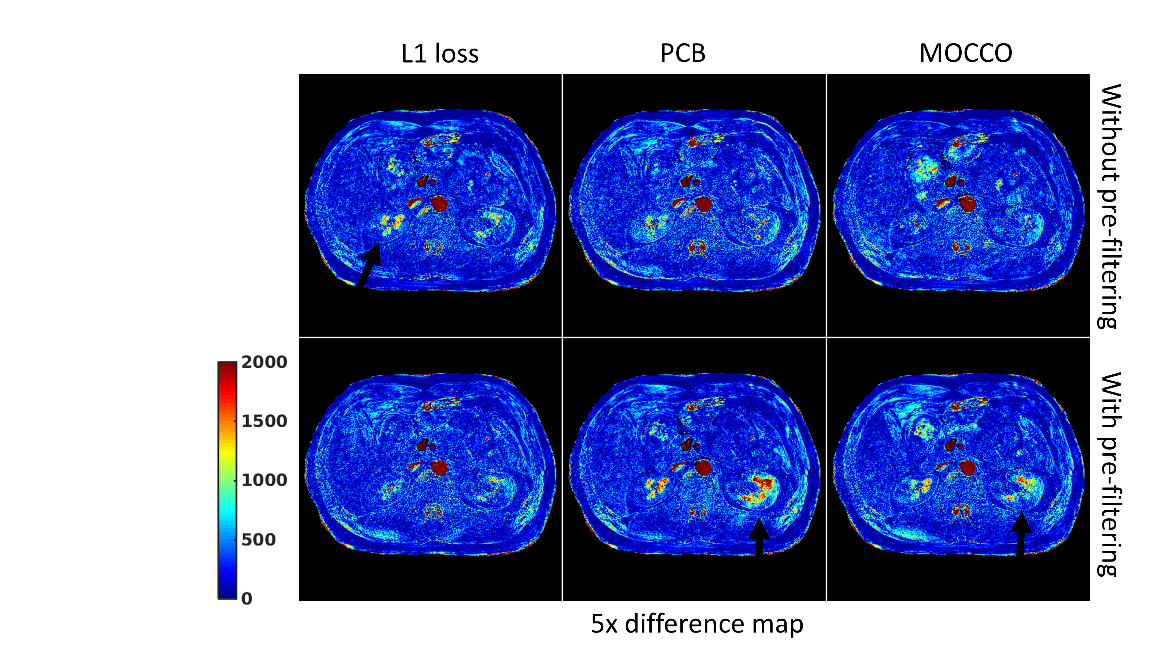
reconstructions that resolve the underlying structure of the liver and the kidneys. Fig.3 shows difference maps w.r.t. the target T1 map obtained by the NLR3D approach. The black arrows in the figure illustrate the substantial errors in the left and right kidneys. For the L1 loss network, pre-subspace filtering mitigates the estimation errors. But for the networks with PCB and MOCCO losses, pre-subspace filtering results in increased error. Fig.4
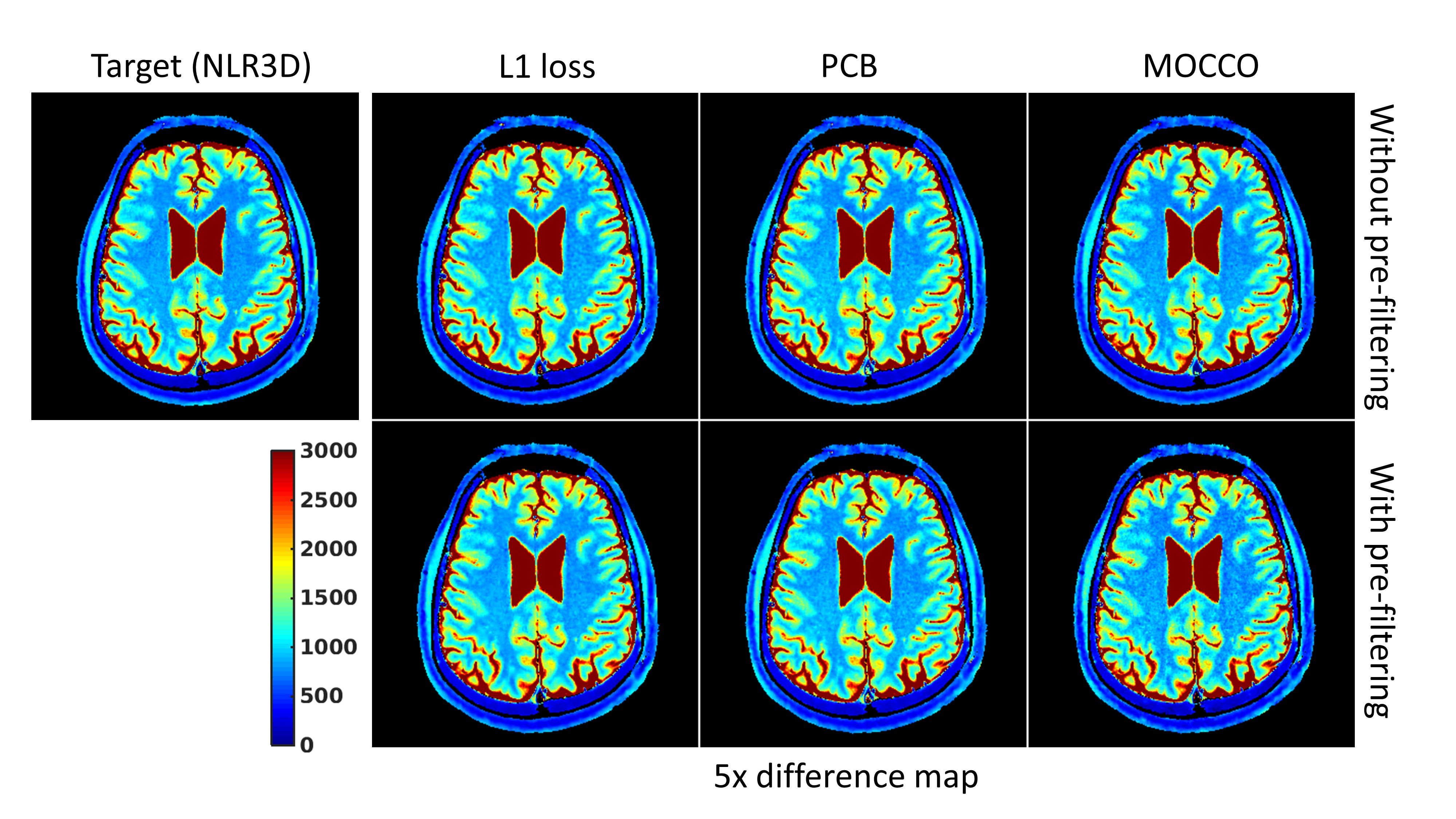
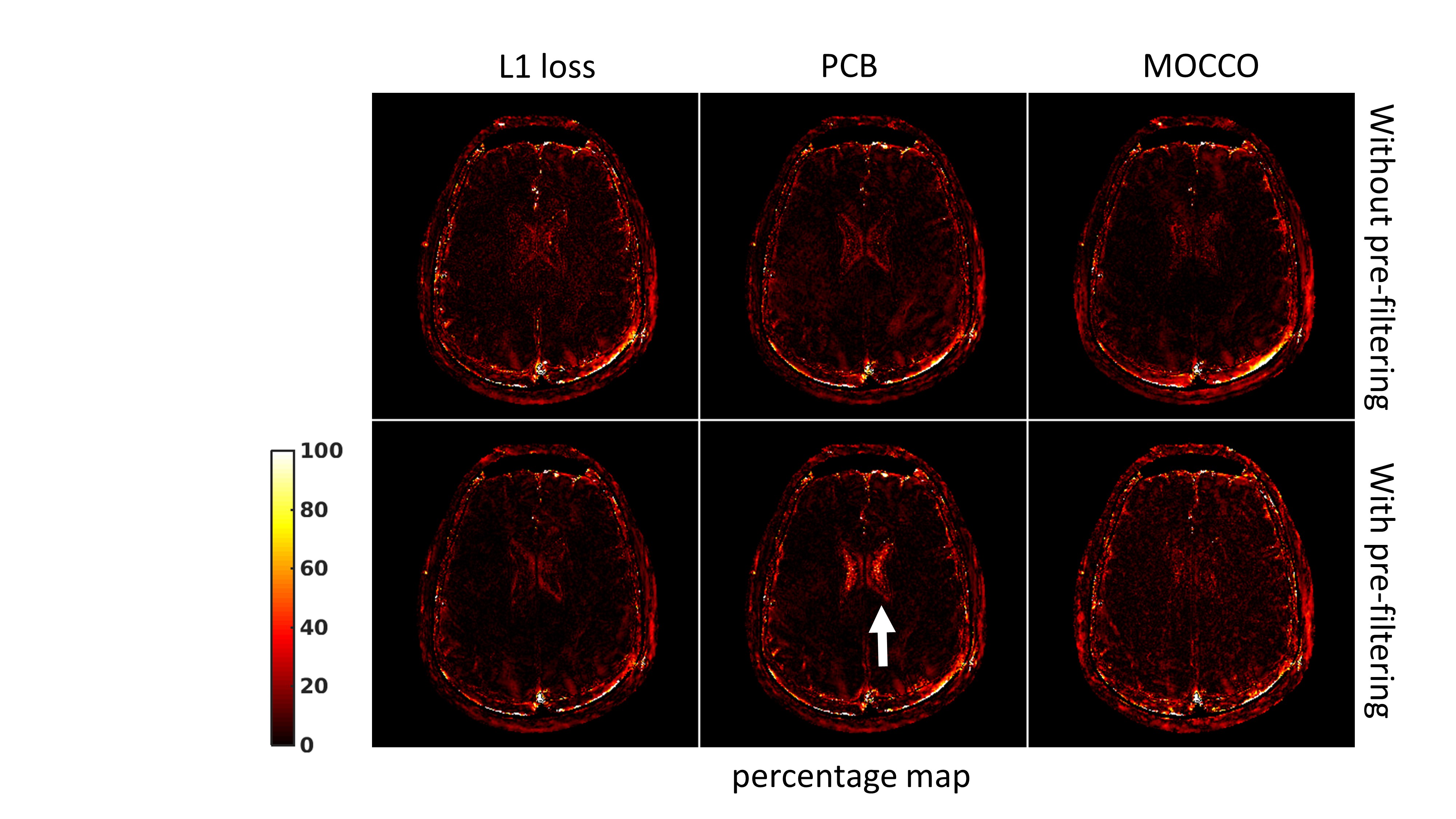
shows the brain T1 mapping results. Networks trained with different losses and
preprocessing steps give similar T1 maps compared to the reference method. In Fig.5, the white arrow indicates that pre-filtering leads to
significant T1 estimation error in CSF for the network trained with the PCB
loss. Additional pre-filtering results in noise amplification on T1 map using the network trained with the MOCCO loss. Conclusion
Relaxation signal model driven constraints were proposed for deep learning based parameter mapping. Results using T1 mapping experiments show model constraints can improve T1 estimation for deep parameter mapping. These constraints can be incorporated either as a pre-processing step or into the loss function.Acknowledgements
The authors would like to acknowledge support from the Arizona Biomedical Research Commission (Grant ADHS14-082996) and the Technology and Research Initiative Fund (TRIF) Improving Health Initiative.References
1. Doneva, M., Börnert, P., Eggers, H., Stehning, C., Sénégas, J., & Mertins, A. (2010). Compressed sensing reconstruction for magnetic resonance parameter mapping. Magnetic Resonance in Medicine, 64(4), 1114-1120.
2. Huang, C., Graff, C. G., Clarkson, E. W., Bilgin, A., & Altbach, M. I. (2012). T2 mapping from highly undersampled data by reconstruction of principal component coefficient maps using compressed sensing. Magnetic resonance in medicine, 67(5), 1355-1366.
3. Zhao, Bo, et al. Accelerated MR parameter mapping with low‐rank and sparsity constraints. Magnetic resonance in medicine 74.2 (2015): 489-498.
4. Velikina, J. V., & Samsonov, A. A. (2015). Reconstruction of dynamic image series from undersampled MRI data using data‐driven model consistency condition (MOCCO). Magnetic resonance in medicine, 74(5), 1279-1290.
5. Tamir, J. I., Uecker, M., Chen, W., Lai, P., Alley, M. T., Vasanawala, S. S., & Lustig, M. (2017). T2 shuffling: Sharp, multicontrast, volumetric fast spin‐echo imaging. Magnetic resonance in medicine, 77(1), 180-195.
6. Fu, Z., Mandava, S., Keerthivasan M.B., Martin D.R., Altbach M.I., Bilgin A. (2018, June) A Multi-Scale Deep ResNet for MR Parameter Mapping, Proc. of ISMRM 2018
7. Fu, Z., Mandava, S., Keerthivasan M.B., Li Z., Martin D.R., Altbach M.I., Bilgin A. (2018, October) MR Parameter Mapping using Sequential Multi-Contrast Acquisitions and Multi-Input Multi-Scale ResNet. ISMRM Workshop on Machine Learning, Part II
8. Cai, C., Wang, C., Zeng, Y., Cai, S., Liang, D., Wu, Y., ... & Zhong, J. (2018). Single‐shot T2 mapping using overlapping‐echo detachment planar imaging and a deep convolutional neural network. Magnetic resonance in medicine.
9. Liu, F., Feng, L., & Kijowski, R. (2018, October) MANTIS: Model-Augmented Neural neTwork with Incoherent k-space Sampling for efficient estimation of MR parameters. ISMRM Workshop on Machine Learning, Part II
10. web.eecs.umich.edu/~fessler/irt
11. Mandava S., Keerthivasan M.B., Martin D.R., Altbach M.I., Bilgin A. (2018, June) Higher-order subspace denoising for improved multi-contrast imaging and parameter mapping. Proc. of ISMRM 2018 12. Liang, Z. P. (2007, April). Spatiotemporal imagingwith partially separable functions. In Biomedical Imaging: From Nano to Macro, 2007. ISBI 2007. 4th IEEE International Symposium on (pp. 988-991). IEEE.
13. Pedersen, H., Kozerke, S., Ringgaard, S., Nehrke, K., & Kim, W. Y. (2009). k‐t PCA: temporally constrained k‐t BLAST reconstruction using principal component analysis. Magnetic resonance in medicine, 62(3), 706-716.
14. Li, Z., Bilgin, A., Johnson, K., Galons, J. P., Vedantham, S., Martin, D. R., & Altbach, M. I. (2018). Rapid High‐Resolution T1 Mapping Using a Highly Accelerated Radial Steady‐state Free‐precession Technique. Journal of Magnetic Resonance Imaging.
15. Paszke, A., Gross, S., Chintala, S., Chanan, G., Yang, E., DeVito, Z., ... & Lerer, A. (2017). Automatic differentiation in pytorch.
Figures