4545
A fast method for field map calculation in multispectral imaging near metal implants1UIH America, Houston, TX, United States
Synopsis
Multispectral acquisition is an important technique for MRI near metal. It is critical to estimate the field map and correct for displacements among bin images before bin combination in order to eliminate blurring. However, current field-estimation methods are either susceptible to noise or are computationally intensive, limiting their clinical applications. We propose a robust and efficient algorithm for calculating the field map from multispectral datasets based on a previous matched-filter field estimation technique. The proposed technique was tested on a digital phantom and generated accurate field maps and high quality images with a very short calculation time.
Introduction
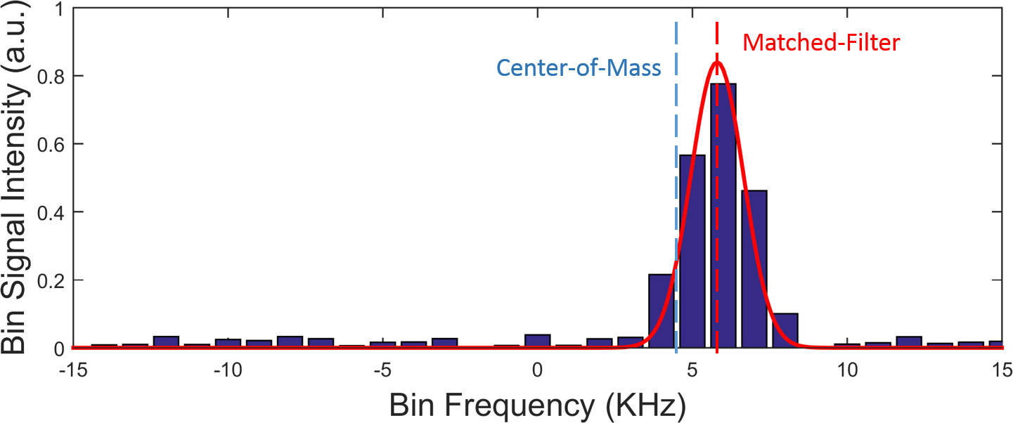
Metal implants disturb the B0 field and cause artifacts in MRI. Multispectral imaging techniques, such as MAVRIC1 and MAVRIC-SL2, have been proposed to suppress artifacts and improve image quality. However, it is necessary to calculate the field from spectral-bin images and correct for their relative displacements before bin combination to avoid blurring2. Two methods have been proposed for field estimation. The center-of-mass (CM) method is straightforward and fast, but suffers from frequency biases especially for noisy data (Fig.1). The matched-filter (MF) approach overcomes this problem. However, it has a high computational cost and takes 1-2 hours to reconstruct typical MAVRIC-SL datasets3, which may limit its clinical applications. We propose an alternative method for field estimation, which is robust against noise and computationally efficient.Methods
The previous MF method has two steps. It first roughly estimates the field by matching the signal intensity across bins to the RF profile (Fig.1), and then accounts for displacements among bin images by a fine search of the field that maximizes the goodness-of-fit, which is defined as:
$$g(x,y,z,f)=1-\frac{|\overrightarrow{S}(x,y,z,f) - \alpha \overrightarrow{RF}(f)|_2}{\alpha |\overrightarrow{S}(x,y,z)|_2|\overrightarrow{RF}(f)|_2} \, ,\: \textrm{with} \: \overrightarrow{S}(x,y,z,f) = [s_1(x - \frac{f-F_1}{BW}) \quad s_2(x - \frac{f-F_2}{BW}) \quad \cdots \quad s_n(x - \frac{f-F_n}{BW})] \, ,$$
where $$$\alpha$$$ is a scalar chosen to match the magnitudes, $$$F_i$$$ and $$$s_i$$$ are bin frequencies and images. Since image interpolation is needed for updating $$$\overrightarrow{S}$$$ in every iteration step for all frequency bins, this method is computationally intensive.
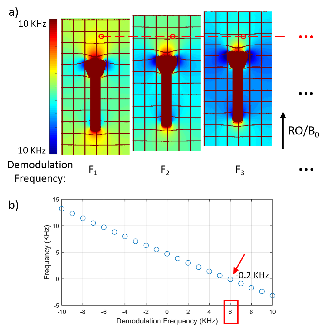
We propose a variant of the MF approach that avoids interpolation and is computationally efficient (MF-Fast). Workflow of MF-Fast is shown in Fig.2. Firstly, original bin images are properly shifted along the RO direction so that they are all aligned (but distorted), which is equivalent to demodulating different acquisitions at the same frequency ($$$F_0$$$). Secondly, a field map (still distorted) is efficiently calculated using the aligned bin images by finding the maximum correlation between the RF profile and signal intensity across bins. Thirdly, field maps corresponding to demodulation at different bin frequencies are generated by shifting the previous one demodulated at $$$F_0$$$ along the RO direction and adding global offsets according to $$$f_b(x,y,z)=f_0(x-\frac{F_b - F_0}{BW},y,z) + (F_b-F_0)$$$, where $$$f_b$$$ and $$$f_0$$$ are voxel frequencies corresponding to demodulation frequencies $$$F_b$$$ and $$$F_0$$$, and RO is along the x direction. Finally, we search for the frequency closest to 0 across bins for each voxel, and add the corresponding bin frequency to generate the final field map:
$$b = \underset{b}{\operatorname{argmin}} \,abs(f_b (x,y,z)) \, ,\textrm{and} \: f(x,y,z) = f_b(x,y,z) + F_b \, ,$$
where b indicates the frequency bin closest to the frequency of voxel (x, y, z) , $$$F_b$$$ is the bin frequency and $$$f_b$$$ is the voxel frequency relative to $$$F_b$$$. The final field map is distortion free because each voxel is effectively demodulated at the closest bin frequency.
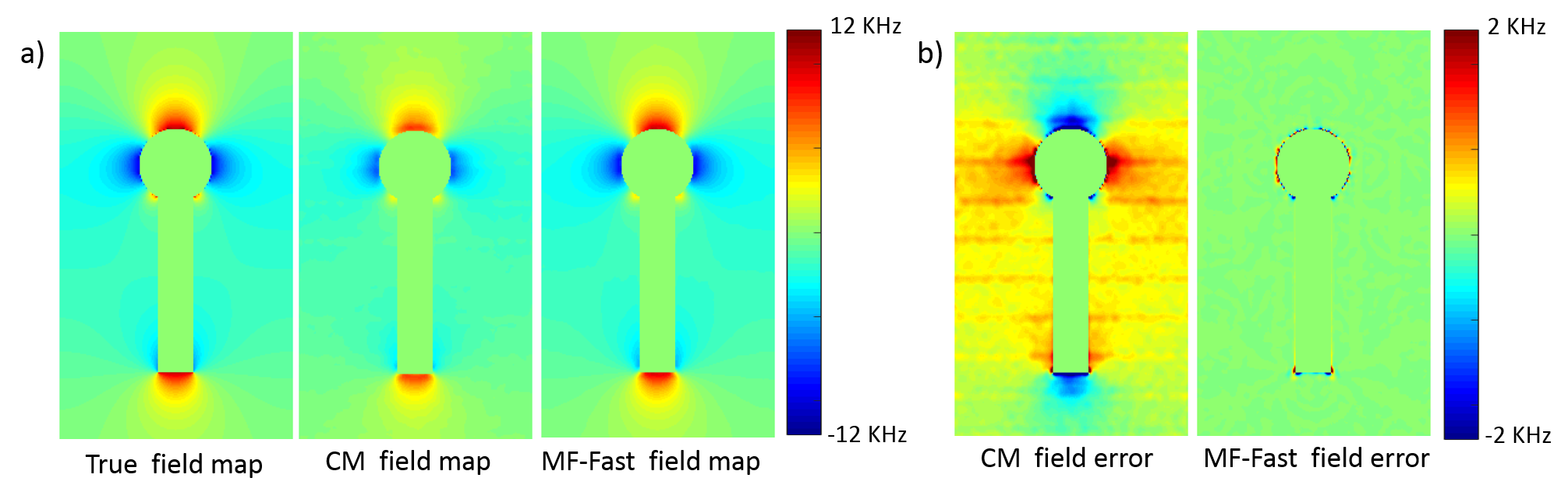
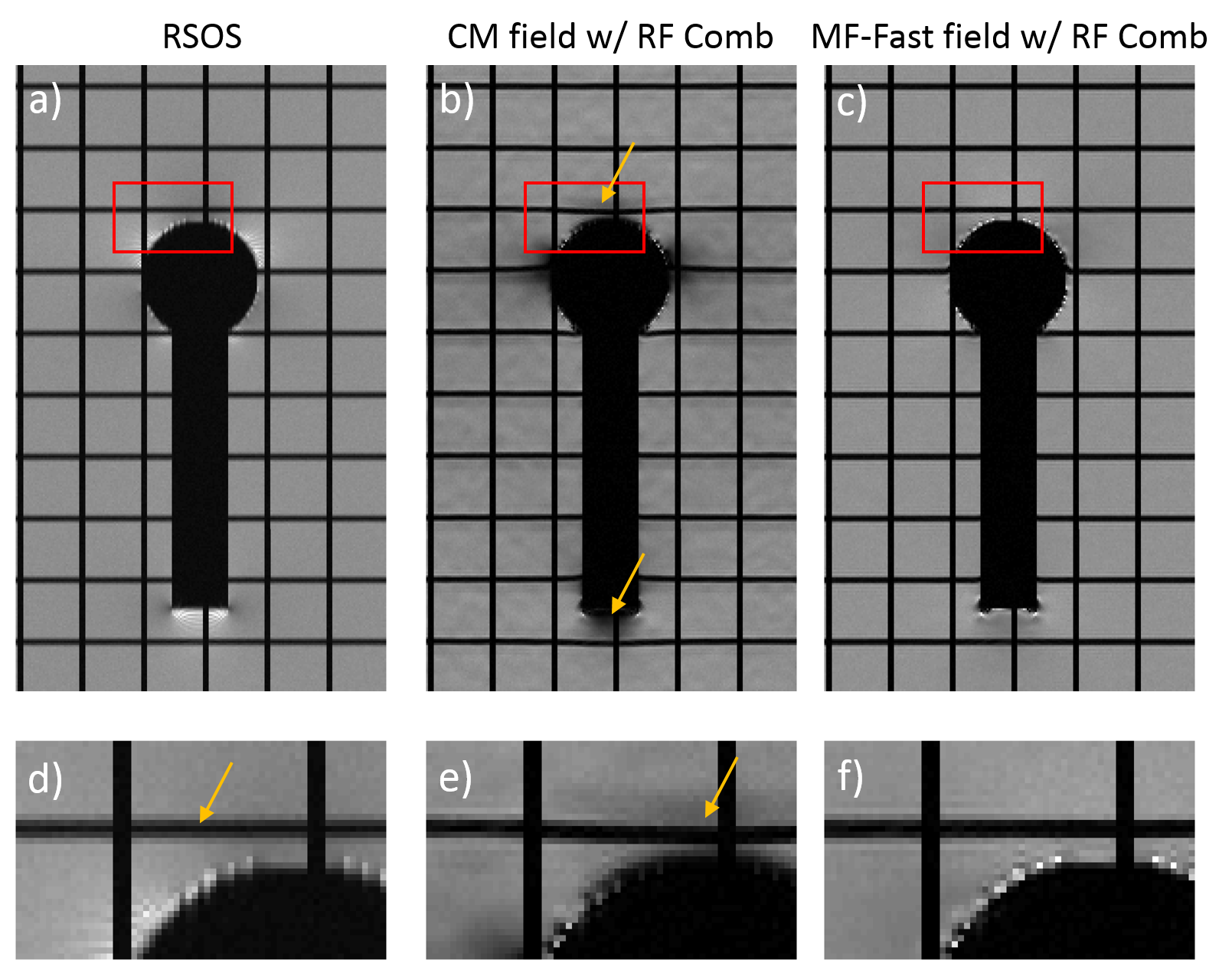
A digital phantom containing a titanium inclusion (χ=182ppm4) was used to demonstrate MF-Fast at 3T. The true field map was calculated using the dipole model5. Effects of the B0 field perturbation were considered in simulation of the MRI signal. 30 Spectra bins from -14KHz to 15KHz with a step size of 1KHz were collected with BW=1KHz/pixel, and the matrix size=384x192. A Gaussian profile was assumed for the RF with a FWHM of 2KHz. Gaussian noise with an SNR of 50 was added to the bin images. Both CM and MF-Fast were used to calculate the field maps, which were subsequently used to correct for displacements among bin images2. The final images were generated using RF-weighted spectral bin combination3 (RF Comb). We also reconstructed the same dataset using direct root-sum-of-squares (RSOS) bin combination for comparison.
Results
Fig.3a shows field maps demodulated at different bin frequencies. The final field for each pixel was determined as shown in Fig.3b. Fig.4a compares the true field map with the ones determined using CM and MF-Fast. Errors of the calculated fields are shown in Fig.4b. The MF-Fast field map is significantly more accurate than the CM field map. Images reconstructed by RSOS bin combination, MF-Fast with RF Comb, and CM with RF Comb are shown in Fig.5. The MF-Fast with RF Comb image has better overall quality, with less blurring, signal voids and distortions. With MF-Fast, the field map calculation only took less than 4 seconds per slice using 8 MATLAB parallel threads.Discussion and Conclusion
We have proposed the MF-Fast method for accurately calculating the field map from multispectral imaging datasets with high computational efficiency. The proposed technique was demonstrated on a digital phantom with a metal inclusion, and generated faithful field maps and high-quality images within a practical reconstruction time. A close comparison between MF-Fast and the previous MF field estimation technique3 is planned for future work.Acknowledgements
No acknowledgement found.References
- Koch KM et. al., A multispectral three-dimensional acquisition technique for imaging near metal implants, Magn Reson Med. 2009 Feb;61(2):381-90.
- Koch KM et. al., Imaging near metal with a MAVRIC-SEMAC hybrid, Magn Reson Med. 2011 Jan;65(1):71-82.
- Quist B et. al., Improved field-mapping and artifact correction in multispectral imaging, Magn Reson Med. 2017 Nov;78(5):2022-2034, Magn Reson Med. 2017 Nov;78(5):2022-2034.
- Schenck JF, The role of magnetic susceptibility in magnetic resonance imaging: MRI magnetic compatibility of the first and second kinds, Med Phys. 1996 Jun;23(6):815-50.
- J.P. Marques et. al., Application of a Fourier‐based method for rapid calculation of field inhomogeneity due to spatial variation of magnetic susceptibility, Concepts Magn Reson 2005:25B:65-78.
Figures