Synopsis

MR-STAT is a framework for obtaining multi-parametric quantitative MR maps using data from single short scans. A large-scale optimization problem is solved in which spatial localisation of signal and estimation of tissue parameters are performed simultaneously by directly fitting a Bloch-based volumetric signal model to the time domain data. In the current work, we exploit sparsity that is inherently present in the problem when using Cartesian sampling strategies to achieve an order of magnitude acceleration in reconstruction times. The new method is tested on synthetically generated data and on in-vivo brain data.

Introduction

MR-STAT¹ is a framework for obtaining multi-parametric quantitative MR maps using data from single short scans. A large-scale optimization problem is solved in which spatial localisation of signal and estimation of tissue parameters are performed simultaneously by directly fitting a Bloch-based volumetric signal model to the time domain data. In previous work,² a highly parallelized, matrix-free Gauss-Newton reconstruction algorithm was presented that can solve the large-scale optimization problem for high-resolution scans. In the current work, we exploit sparsity that is inherently present in the problem when using Cartesian sampling strategies to achieve an order of magnitude acceleration in reconstruction times.

Theory

In MR-STAT, parameter maps are obtained by iteratively solving

$$\hat{\alpha} = \text{argmin}_\alpha \frac{1}{2}\left\lVert d-s(\alpha)\right\rVert ^2_2,$$

where $$$d$$$ is the measured data, $$$s$$$ is a Bloch-equation based signal model and $$$\alpha$$$ are the parameter maps concatenated into a single vector. In previous work² a Gauss-Newton (GN) method was proposed that, at each iteration, obtains an update step $$$p$$$ in parameter space by iteratively solving the linear system $$J^TJp=-g,$$ where $$$g$$$ is the gradient of the objective function and $$$J$$$ is the Jacobian matrix (matrix of partial derivatives of the residual vector w.r.t. each parameter). It was observed that, while the matrix $$$J$$$ itself is too large to store into computer memory, only matrix-vector products of the form $$$Jv$$$ and $$$J^Tv$$$ are needed to solve the linear system. However, this "matrix-free GN-method" requires re-computation of the entries of $$$J$$$ for each matrix-vector product, which forms the computational bottleneck of the reconstruction algorithm.

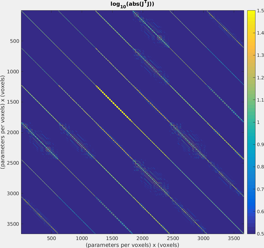
In this work we hypothesize that $$$J^TJ$$$ admits a sparse, banded structure when using Cartesian acquisitions with smoothly varying flip angles. For such acquisitions, the point spread function, which encapsulates dependencies between voxels, is spatially mostly confined to the phase-encoding direction and limited in width. Hence $$$J^TJ$$$, which also contains these spatial dependencies, is expected to contain mostly zeros. In figure 1, this is confirmed to be the case for a small scale numerical example. Given that $$$J^{T}J$$$ is a sparse, banded matrix, it can be computed and stored upfront (once per outer iteration). Subsequent multiplications with $$$J^TJ$$$ are computationally inexpensive and hence $$$p$$$ can be obtained rapidly in this "sparse GN-method".

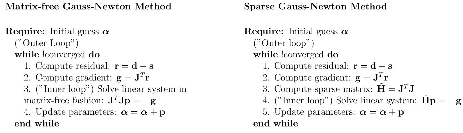
In figure 2, pseudo-algorithms for both the matrix-free and sparse GN reconstruction methods are presented.

Methods

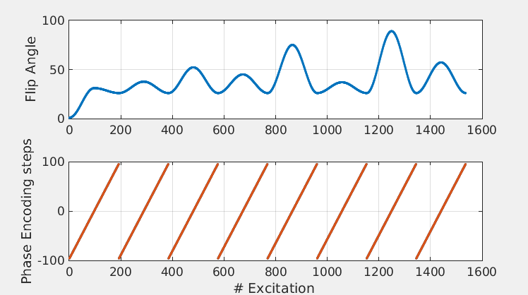
The reconstruction methods were compared on synthetically generated data and on in-vivo brain data. In both cases, a 2D gradient-balanced, transient-state pulse sequence was used with a flip angle that smoothly varies each TR and a linear, Cartesian k-space filling, as shown in figure 3. For the synthetic experiment, the sequence was used to simulate data with a (simulated) scan time of 7.8 seconds. For the in-vivo brain experiment, the transient-state sequence was implemented on a 1.5 Philips-Ingenia MR-System and was used to scan a healthy volunteer with a 13-channel receive head-coil. The scan time was 6.8 seconds with a scan resolution of 1x1x5mm³.

From the simulated/acquired data, $$$T_1,T_2,B_1^+,\Delta B_0,\rho$$$ maps were reconstructed. For the matrix-free GN-method, the number of inner iterations was limited to 10 because of time constraints. For the sparse GN-method, 15 subdiagonals were computed for each parameter pair, resulting in storage of ~0.04% needed compared to the full matrix size for the in-vivo brain dataset. The reconstruction algorithms were written in the Julia programming language³ and were run on a computing cluster using 64 cores.

Results

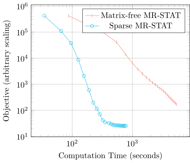
In figure 3, convergence curves for the matrix-free and the sparse GN-methods are shown. For both methods the parameter maps converge to the true maps but the reconstruction time for the sparse GN-method is decreased by an order of magnitude.

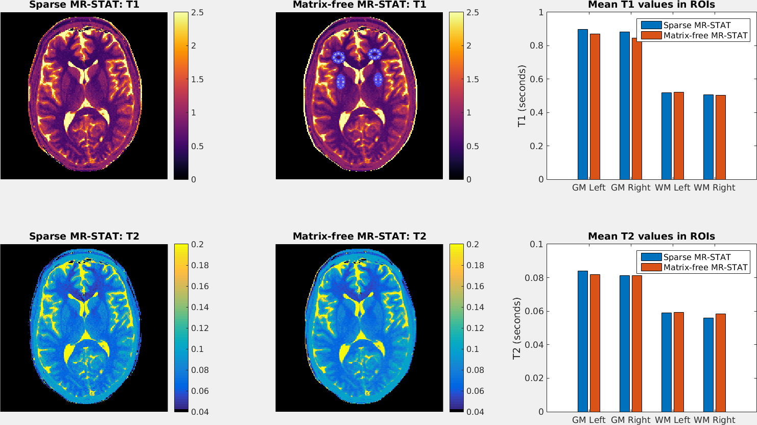
Figure 4 shows the reconstructed in-vivo T1 and T2 maps for the sparse GN-method and a comparison with the matrix-free GN-method. Using the sparse GN-method the reconstruction time was ~50 minutes whereas for the matrix-free GN-method it was ~320 minutes.

Discussion

Even though in the sparse GN-method an approximation of $$$J^TJ$$$ is used (which itself approximates the Hessian matrix), the optimization algorithm converges to the same parameter maps. In fact, the method can even lead to better update steps (as seen in figure 3) because the number of iterations for the inner loop is not limited, allowing it to better take into account the curvature of the objective function.

For non-Cartesian sampling strategies $$$J^TJ$$$ will have a more complicated structure and will be much less sparse, but using sparse approximations (directly or as preconditioner) might still result in sufficiently good update steps $$$p$$$ and is subject to further study.

Conclusion

Acknowledgements

References

[1] Sbrizzi A, van der Heide O, Cloos M, van der Toorn A, Hoogduin H, Luijten PR, van den Berg CAT. Fast quantitative MRI as a nonlinear tomography problem. Magnetic Resonance Imaging, 46:56–63, 2018.3.

[2] van der Heide O, Sbrizzi A, Luijten PR, van den Berg CAT. Proc. 26th Sci. Meet. Int. Soc. Magn. Reson. Med. Paris, 2018:0266.

[3] Bezanson J, Edelman A, Karpinski S, Shah VB. Julia: A fresh approach to numerical computing. CoRR, abs/1411.1607, 2014.