Introduction

MR fingerprinting (MRF) offers a rapid way to simultaneously quantify multiple tissue parameters. By varying acquisition parameters over a time-series of images, e.g., flip angles (FA) and repetition times (TR), tissue-specific signals, i.e., fingerprints, are obtained ¹. To make the MRF technique most suitable for clinical needs, efforts are still to be made to accelerate MRF acquisitions while maintaining the accuracy in parameter determination.

Methods

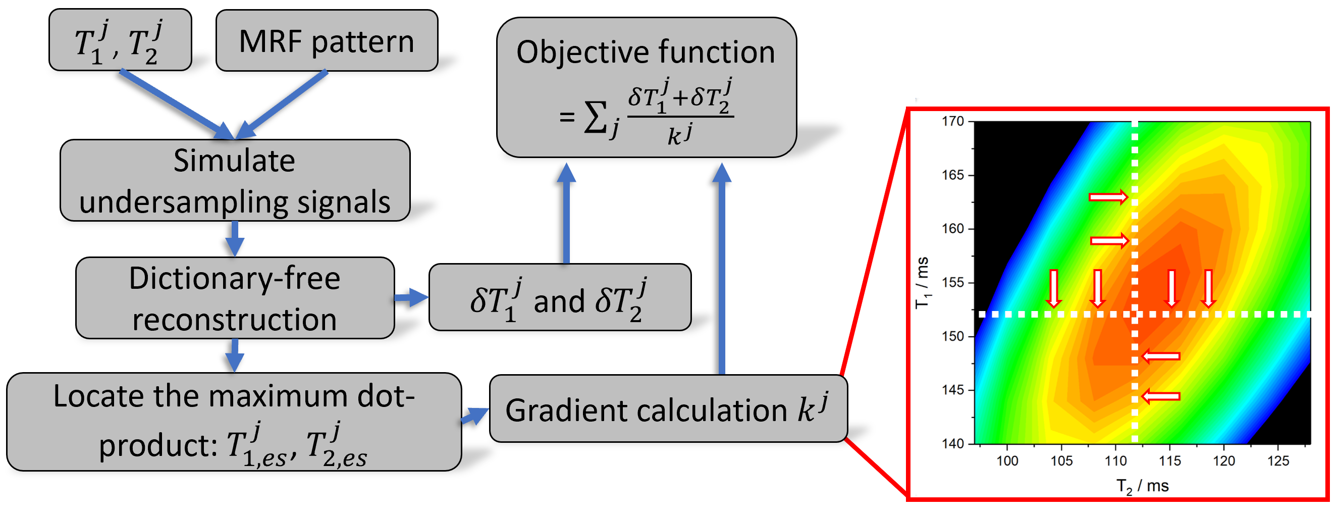
In our optimization framework, FA patterns were generated by the trigonometric interpolation method ³. TRs were kept in a constant fashion throughout each of simulated MRF acquisitions. As can be seen in Figure 1, the tissue which modeled by $$$T^j_1$$$ and $$$T^j_2$$$ was inserted together with a candidate MRF pattern into the EPG simulator ⁵. Gaussian noise, i.e., SNR = 4.0, was added to both the real and the imaginary part of the signal to mimic the signal gathered from an undersampling acquisition ⁸. The amplitude of Gaussian noise was modulated by the signal magnitude throughout the fingerprinting train ⁸. A DFR was performed on the noisy fingerprint to retrieve the best matching $$$T^j_{1,es}$$$ and $$$T^j_{2,es}$$$. The corresponding estimation biases $$$\delta T^j_{1/2}$$$ was computed according to $$$\frac{\left| T^j_{1/2} - T^j_{1/2,es} \right |}{T^j_{1/2}}$$$. In addition, the similarity of the best matching fingerprint ($$$DP^j_{max}$$$) to its adjacent $$$T_1$$$ and $$$T_2$$$ entires ($$$DP^j_i$$$) was minimized in order to alleviate the matching ambiguity. We quantified the similarity by a calculating gradients $$$k_j$$$ in the $$$T_1-T_2$$$ space ² (Figure 1): $$\begin{split} &k^j = \sum_{i=1}^{4}\frac{\Delta DP^j_i}{\Delta T^j_{1,i}} + w\sum_{i=1}^{4}\frac{\Delta DP^j_i}{\Delta T^j_{2,i}}, \\ &\Delta DP^j_i = DP^j_{max} - DP^j_i, \\ &\Delta T^j_{1/2,i} = T^j_{1/2,es} - T^j_{1/2,i}. \end{split} $$ We set the weighting factor $$$w = 10^3$$$ for increasing the $$$T_2$$$ accuracy in our optimization. In Figure 1, eight entries ($$$T^{step}_1 = 5ms$$$, $$$T^{step}_2 = 2.5ms$$$) around the best matching entry, e.g. $$$DP^j_{max}$$$, were involved in the gradient calculation. We defined the total objective function $$$p$$$ as: $$ p = \sum_{j} \frac{\delta T^j_1 + \delta T^j_2}{k^j}. $$ It sums over contributions from all tissue components in the anatomical region of interest. The parallel tempering algorithm ⁶ was used to minimize the proposed objective function $$$p$$$. In-vivo data was acquired on a $$$3T$$$ MRI scanner ($$$Achieva \;3T$$$, Philips, The Netherlands). $$$36$$$ constant density spiral interleaves were combined to fully sample the k-space. A non-uniform dictionary with $$$T_1$$$ resolutions of $$$40 ms$$$ ($$$T_1 \in [100 ms, 2000 ms]$$$), $$$200 ms$$$ ($$$T_1 \in [2010 ms, 6000 ms]$$$) and $$$T_2$$$ resolutions of $$$20 ms$$$ ($$$T_2 \in [10 ms, 500 ms]$$$), $$$200 ms$$$ ($$$T_2 \in [510 ms, 2500 ms]$$$) were used for reconstruction.

Results and discussion

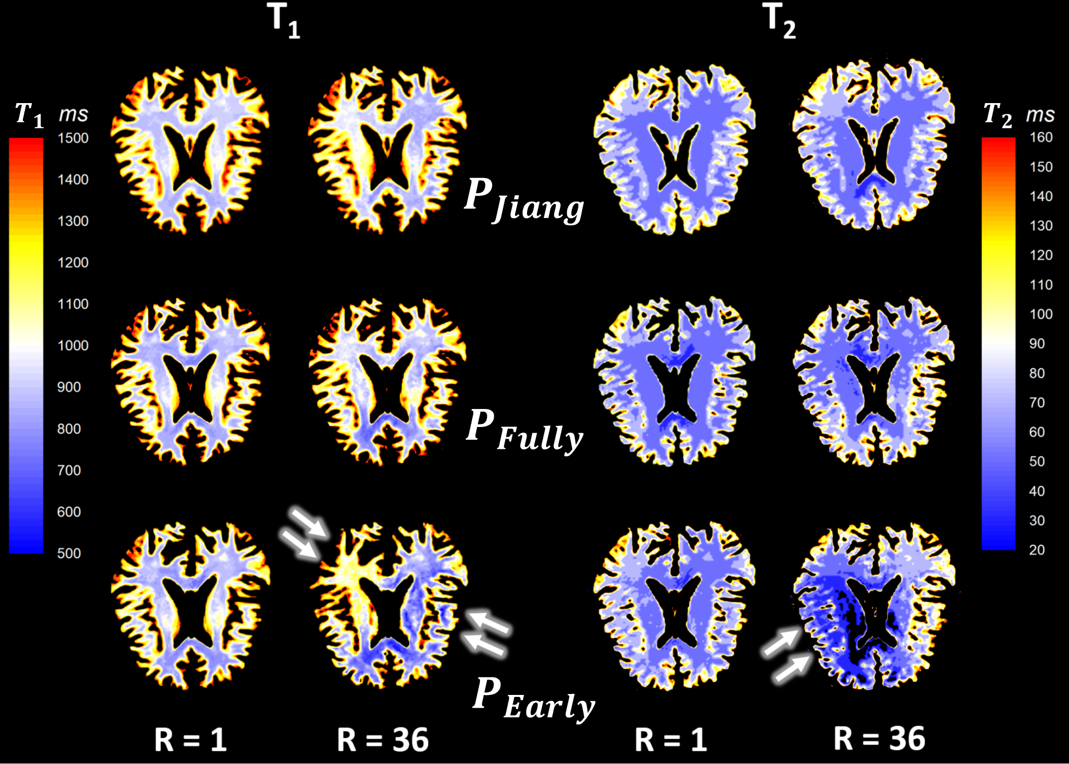
We compare the encoding performance of Jiang's pattern $$$P_{Jiang}$$$ ⁷, our algorithm pattern $$$P_{Fully}$$$ (Fully: fully converged), and an algorithm pattern $$$P_{Early}$$$ (Early: early stopping). The proposed algorithm is able to generate MRF patterns such as (A) in Figure 2, by including a priori knowledge, i.e., the relaxation times of tissues found in the brain (Figure 2 (B)). By comparing $$$T_{1/2}$$$ maps under fully sampled (R=1) and undersampled (R=36) measurements (Figure 3), $$$P_{Fully}$$$ shows an equivalent undersampling tolerance to $$$P_{Jiang}$$$ ⁷. Previous MRF measurements ^1,7 showed large inaccuracies in the CSF $$$T_2$$$ prediction. We visualize inconsistencies in CSF estimation in Figure 4 by thresholding the quantitative maps. The distribution of CSF can be retrieved from the $$$T_1$$$ maps due to the higher precision in CSF $$$T_1$$$ estimations ¹. Notably, in the measurement obtained with $$$P_{Jiang}$$$, the common circulation area of CSF such as lateral ventricles and brain sinuses are invisible due to their low reconstructed $$$T_2$$$ values (marked by white arrows in Figure 4). However, CSF $$$T_2$$$ maps from the $$$P_{Fully}$$$ acquisition (second row in Figure 4) better represent the CSF distribution. As predicted by the optimization cost function, the corresponding quantitative maps reconstructed from the $$$P_{Fully}$$$ measurements show consistent CSF distribution between $$$T_1$$$, $$$T_2$$$ maps, even for high undersampling of R=36. On the other hand, weaker robustness to undersampling, i.e., inconsistencies in $$$T_1$$$ and $$$T_2$$$ maps (last row in Figure 4), are observed in the measurements with $$$P_{Early}$$$. When thresholding for GM and WM, $$$P_{Jiang}$$$ and $$$P_{Fully}$$$ measurements show similar results. However, reconstructed maps from $$$P_{Early}$$$ measurements (last row of Figure 5) show $$$T_1$$$ overestimation (underestimation) in the left (right) part of the WM region (indicated by arrows in Figure 5). In addition, a more noisy $$$T_2$$$ map is observed in the $$$P_{Early}$$$ reconstructed $$$T_2$$$ maps.

Conclusion

The proposed optimization framework enables optimized MRF pattern generation based on tissues of interest for accurate quantitative MR mappings.

References

1. Dan. M, et al. Magnetic Resonance Fingerprinting. Nature. 2013; 495: 187-193.
2. Tianyu. H, et al. Fast Dictionary-free Reconstruction in MR Fingerprinting. Proc. Intl. Soc. Mag. Reson. Med. 2018; 26: 2893.
3. Kendall A, An Introduction to Numerical Analysis (2nd edition), Section 3.8. John Wiley & Sons. New York,1988.
4. Ouri. C, et al. Algorithm comparison for schedule optimization in MR fingerprinting Magnetic Resonance Imaging. 2017; 41:15-21.
5. Matthias W, Extended phase graphs: Dephasing, RF pulses, and echoes ‐ pure and simple. Journal of Magnetic Resonance Imaging. 2015; 41: 266-295.
6. David. J. E, et al. Parallel tempering: Theory, applications, and new perspectives. Phys . Chem. Chem. Phys. 2005; 7: 3910-3916.
7. Yun. J, et al. MR fingerprinting using fast imaging with steady state precession (FISP) with spiral readout. Magn Reson Med. 2015; 74:1621-1631.
8. Karsten S, et al. Towards predicting the encoding capability of MR fingerprinting sequences. Magnetic Resonance Imaging. 2017; 41: 7-14.