4523
Schedule design for parameter quantification in the transient state using Bayesian optimisation1Dipartimento di Informatica, Università di Pisa, Pisa, Italy, 2Stella Maris Scientific Institute and IMAGO7 Research Foundation, Pisa, Italy, 3Dipartimento di Fisica, Università di Pisa, Pisa, Italy, 4Computer Science, Technische Universitat Munchen, Munich, Germany
Synopsis
Magnetic resonance fingerprinting (MRF) is a useful tool for simultaneously obtaining multiple tissue-specific parameters in an efficient imaging experiment. This technique uses transient state acquisitions with pseudo-random acquisition parameters. However, specific schedules may be better suited for certain parameter ranges or sampling patterns. This work aims to introduce a framework for pulse sequence optimization, including aliasing and noise in our estimates, individually or jointly optimizing for T1 and T2 relaxation times. We demonstrated the schedules created by our algorithm using MRI acquisitions on a healthy volunteer. The design framework could improve the efficiency and accuracy of T1 and T2 acquisitions.
Introduction
New methods based on transient-state imaging, including magnetic resonance fingerprinting1 (MRF), have several advantages as they efficiently sample the MR signal and produce quantitative estimates. Despite several accounts looking into optimising such acquisitions2,3,4,5,6, the choice of the parameters of transient-state sequences remains an open problem as the degrees of freedom to design the sequence are nearly unlimited. Here, we propose a framework to optimise T1 and T2 parameters based on Bayesian optimisation algorithms, including aliasing and noise in our estimates. As a demonstration of our framework, we used it to optimally select the varied sequence parameters in an MR Fingerprinting experiment.Methods
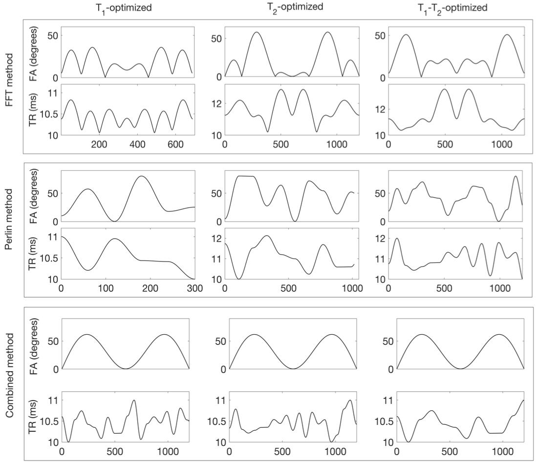
Our optimisation method was based on a Bayesian optimisation algorithm (BO)7,9. We performed a simulation of an SSFP MRF8 signal evolutions with the Extended Phase Graph (EPG) formalism12. To work on a realistic dataset, we used the 100th slice of a numerical phantom brain from the Brainweb database11, where we also included under-sampling artefacts by applying forward and backward non-uniform Fourier transform13 for each frame. Complex white Gaussian noise was added to the raw k-space data. The overall errors of the quantitative maps was used as the cost function (l2 norm of the difference between maps), excluding the background values. We first individually optimised T1 and T2 estimations; then, we optimised for the two parameters simultaneously. In the latter case, we used the sum of the overall errors of T1 and T2 maps as a cost function. We considered three ways of generating the function consisting of m excitations for FA or TR sequences, where the schedule length m was one of the input parameters of our optimisation model:
- FFT method: We used the first coefficients of a Fourier series, zero-padding the remaining to estimate a slow-varying function.
- Perlin method: To produce Perlin noise we generated normally distributed random numbers and interpolated them with a cosine function.
- Combined method: We also used the combination of the two methods described before, using Perlin noise for TR and Fourier coefficients for FA.
The optimised schedules were evaluated in vivo on the brain of a volunteer, using a GE Hdxt 1.5T scanner equipped with an 8ch receive coil (Milwakee, US).
Results
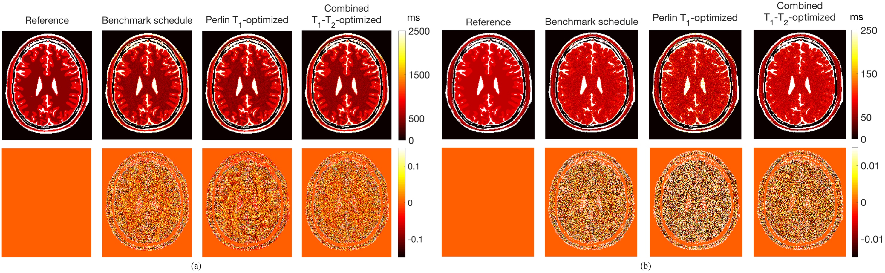
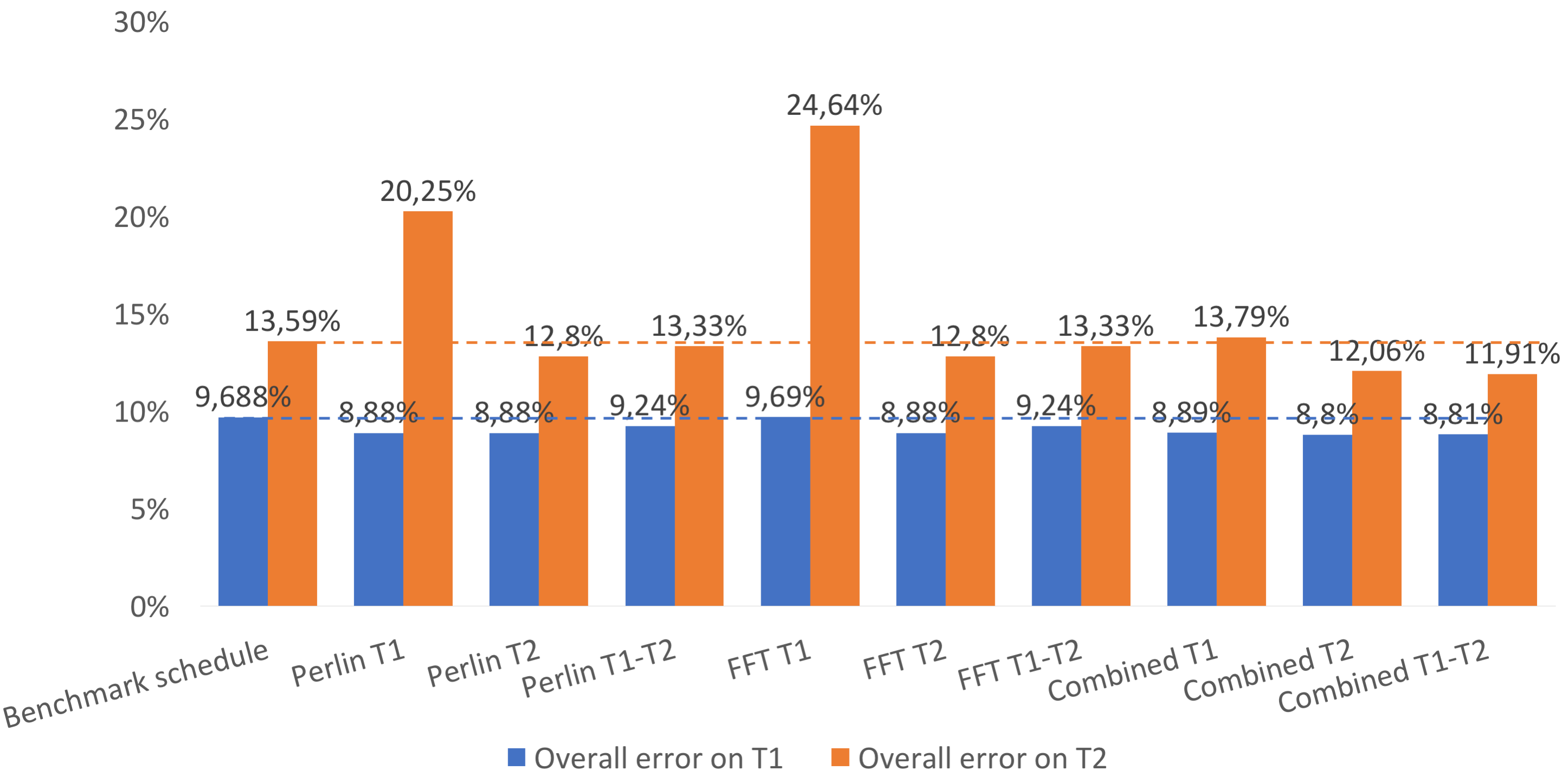
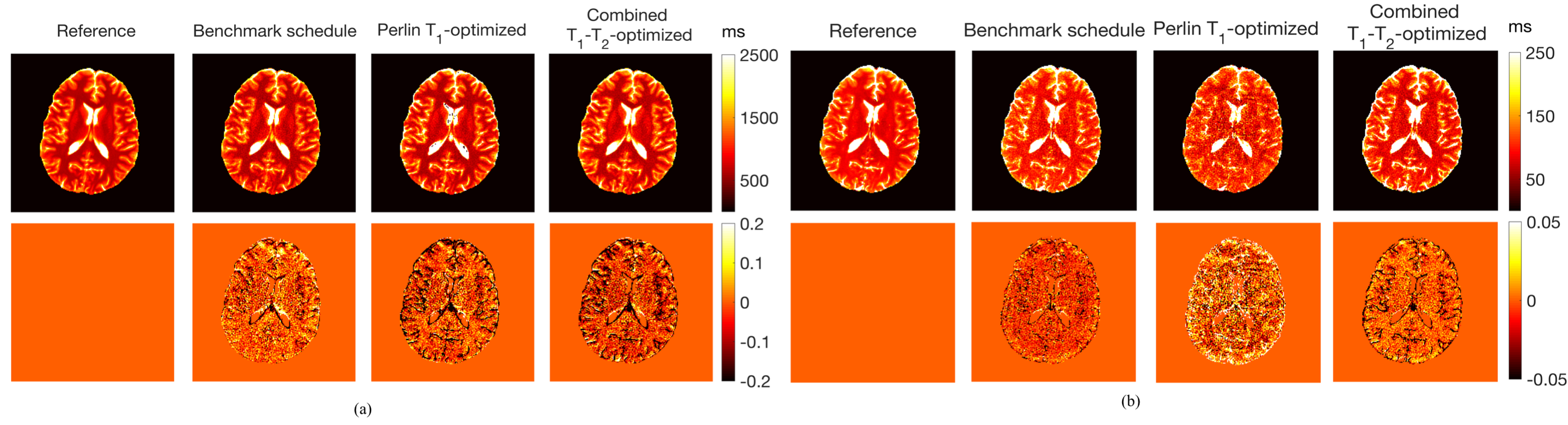
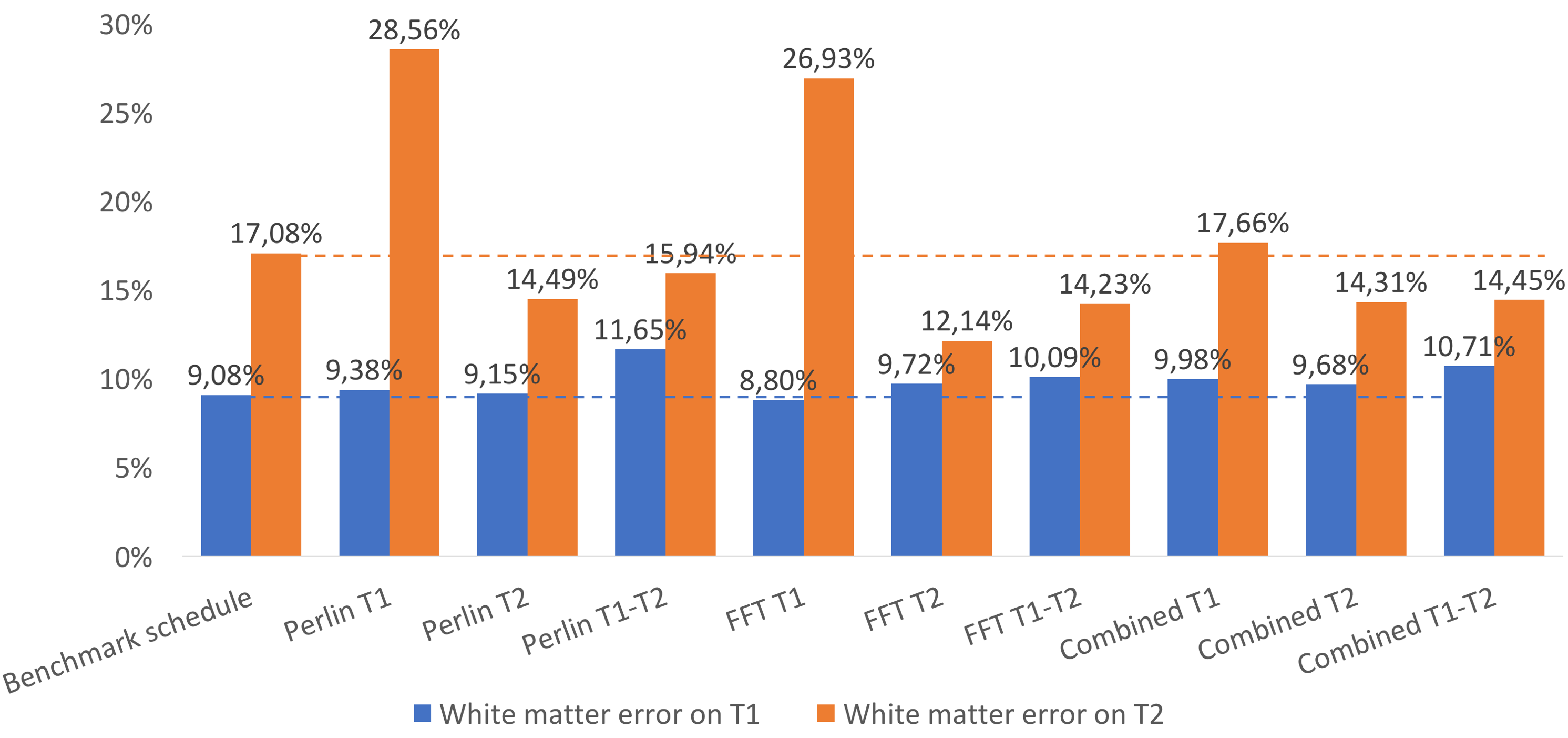
The implemented algorithm converged within 5 to 10 hours depending on the setup. For example, the FFT global optimisation (with iterations) was computed in 300 minutes on an Intel Xeon processor E5-2600 v4. The schedules resulting from our optimisation algorithm are reported in Figure 1. It can be noted that different schedules have different number of excitations, with the runs optimising only T1 resulting in shorter schedules. As seen in other optimisation works in literature3,4,6, the schedules usually start with a few large flip angles within the first pulses after the initial inversion. Figure 2 shows T1 and T2 maps from the simulated experiment as well as the relative error maps (evaluated with respect to the reference data). Figure 3 shows overall errors on parametric maps obtained from simulations. As can be seen, the Perlin method optimised for T1 improved the T1 map at the expense of degrading the accuracy of T2 map. This is due to the short acquisition length of this scheme. Using the schedule obtained from the Combined method optimising both T1 and T2, the accuracy of both maps was improved. Figure 4 shows the reconstructed T1 and T2 maps as well as the relative error maps (evaluated with respect to the reference data). Figure 5 shows all computed errors on the white matter region of parametric maps in the case of the in-vivo experiment. Our optimised schedules did not improve on the accuracy of T1 maps. Instead, almost for all the schedules, the T2 maps accuracy was improved, apart from the ones obtained from individual T1-optimisation.Discussion
Our framework could successfully obtain new MRF schedules in a reasonable timeframe. The timeframe of 300 minutes can be considered reasonable as after one optimisation process, the same schedules can be reused for a large number of MRI scans. The optimised schedules enable slightly better or similar accuracy both for T2 and T1 maps. Remarkably, we found that the optimised acquisition parameters appear to follow acquisition sequence trends already seen3,4,6. In the experiments performed, we manually selected the search space dimension together with the parameters bounds. This provided good performance thanks to the possibility to restrict the search space, allowing a faster convergence to a local minimum.Conclusion
In conclusion, our flexible framework allows the design of acquisition patterns tailored to specific experimental purposes. After further validation, schedules obtained with our method could be used for research studies, with the promise of improving the efficiency and accuracy of quantitative MRI protocols.Acknowledgements
References
[1] D. Ma et al., “Magnetic resonance fingerprinting,” Nature, vol. 495, no. 7440, pp. 187–192, Mar. 2013.
[2] B. Zhao, K. Setsompop, H. Ye, S. F. Cauley, and L. L. Wald, “Maximum Likelihood Reconstruction for Magnetic Resonance Fingerprinting,” IEEE Trans. Med. Imaging, vol. 35, no. 8, pp. 1812–1823, Aug. 2016.
[3] B. Zhaoet al., “Optimal Experiment Design for Magnetic Resonance Fingerprinting: Cramér-Rao Bound Meets Spin Dynamics,” Oct. 2017.
[4] J. Assländer, R. Lattanzi, D. K. Sodickson, and M. A. Cloos, “Relaxation in Spherical Coordinates: Analysis and Optimization of pseudo-SSFP based MR-Fingerprinting,” Magn. Reson. Med., Mar. 2017.
[5] J. Assländer, S. J. Glaser, and J. Hennig, “Pseudo Steady-State Free Precession for MR-Fingerprinting,” Magn. Reson. Med., vol. 77, no. 3, pp. 1151–1161, Mar. 2017.
[6] O. Cohen and M. S. Rosen, “Algorithm comparison for schedule optimisation in MR fingerprinting,” Magn. Reson. Imaging, vol. 41, pp. 15–21, Sep. 2017.
[7] J. Mockus, Bayesian Approach to Global Optimization, vol. 37. Dordrecht: Springer Netherlands, 1989.
[8] Y. Jiang, D. Ma, N. Seiberlich, V. Gulani, and M. A. Griswold, “MR fingerprinting using fast imaging with steady state precession (FISP) with spiral readout,” Magn. Reson. Med., vol. 74, no. 6, pp. 1621–1631, Dec. 2015.
[9] B. Shahriari, K. Swersky, Z. Wang, R. P. Adams, and N. De Freitas, “Taking the human out of the loop: A review of Bayesian optimization,” Proceedings of the IEEE, vol. 104, no. 1. pp. 148–175, Jan-2016.[10] C. Rasmussen and C. Williams, Gaussian Processes for Machine Learning, vol. 14, no. 2. 2006.
[11] D. L. Collins et al., “Design and construction of a realistic digital brain phantom,” IEEE Trans. Med. Imaging, vol. 17, no. 3, pp. 463–468, Jun. 1998.
[12] M. Weigel, “Extended phase graphs: Dephasing, RF pulses, and echoes - pure and simple,” J. Magn. Reson. Imaging, vol. 41, no. 2, pp. 266–295, Feb. 2015.
[13] J. M. Pauly, “Gridding & the NUFFT for Non-Cartesian Image Reconstruction,” ISMRM Educ. Course Image Reconstr., vol. 20, pp. 4–6, 2012.[14] J. I. Hamiltonet al., “MR fingerprinting for rapid quantification of myocardial T 1 , T 2 , and proton spin density,” Magn. Reson. Med., vol. 77, no. 4, pp. 1446–1458, Apr. 2017.
Figures