Synopsis

A comparative analysis between IR-bSSFP and MR Fingerprinting was performed in numerical simulations for single and multi-component parameter mapping. The single component matching works for both methods, although the accuracy for T2 is better for MR Fingerprinting. The multi component matching for a constant flip angle IR-bSSFP sequence can only match to the T1* values and cannot distinguish between the underlying T1/T2 values. Using the MR Fingerprinting sequence with a varying flip angle it is possible to match to the T1/T2 components.

Introduction

In magnetic resonance fingerprinting (MRF) [1] an acquisition scheme with varying pulse sequence parameters is used to enable simultaneous multi-parameter mapping. The original MRF sequence is closely related to the IR-bSSFP approach for simultaneous T₁, T₂, and proton density mapping [2], in which constant flip angle α and TR are applied after an initial inversion and a preparation pulse with α/2 at TR/2, resulting in an exponential signal recovery with an effective relaxation time $$$T_1^*$$$.

Both methods can be applied for the simultaneous estimation of T₁, T₂ and proton density maps. Multi-component analysis for IR-bSSFP has been done based on the effective relaxation time $$$T_1^*$$$ [3] and for MRF based on the T₁ and T₂ values [4,5]. Combined with radial or spiral acquisition with high undersampling and dictionary matching both scans can be performed in a very short scan time. The main difference that remains is the flip angle variation. So what are the advantages of the flip angle variation?

In this work we try to answer this question and investigate the differences between the two sequence types in single component matching and multi-component analysis experiments.

Methods

Four sequences with different FA variations ((1) constant 45°, (2) constant 25°, (3) smooth and (4) high frequency variation) all consisting of 500 measurements with TR=3.6ms were considered (Fig.1). Dictionaries containing the signal evolutions for 6240 T₁/T₂ combinations (T₁ from 5ms to 2s, T₂ from 4ms tot 1s both with an adaptive step size) were computed for each sequence. The exponential signal for a constant FA α is described through the effective relaxation time$$T_1^*=\left(\frac{1}{T_1}\cos^2\alpha+\frac{1}{T_2}\sin^2\alpha\right)^{-1}$$and the signal value in steady-state by the ratio between T₁ and T₂.

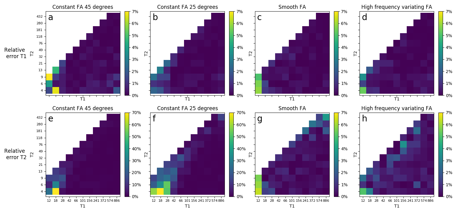
The accuracy and precision of the single component parameter mapping of the four sequences were compared in numerical simulations. 65 test signals with different T₁/T₂ combinations were considered, for each combination one signal with 100 noise realizations was simulated with an SNR of 10. These noisy signals were matched to the dictionary using an inner product matching as proposed in [1]. The quality of the matching was determined by the mean relative error and standard deviation in the mapped relaxation times.

The sequences were further compared in a multi-component matching task. Different mixtures of two T₁ and T₂ relaxation times were tested for different levels of additive Gaussian noise. For each simulated signal the multi-component matching is performed through the non-negative least squares (NNLS) algorithm [6]. This process was repeated 400 times with different noise realizations leading to a distribution of matched components.

The NNLS algorithm finds sparse results [7], which makes it an effective method to obtain a decomposition with a small number of components.

Results

Results from the single component parameter mapping are shown in Fig.2,3 . Sequences 1 and 2 show a reduced accuracy and precision compared to the varying FA sequences for T₂. For most considered T₁/T₂ combinations the error is low (<1%), but it increases for small T₁ and T₂ for every sequence. For the constant FA, the FA influences the precision of the matched relaxation times. Using a smaller FA improves the precision of the T₁ matching and reduces the precision in T₂, which is expected from the relation through $$$T_1^*$$$.

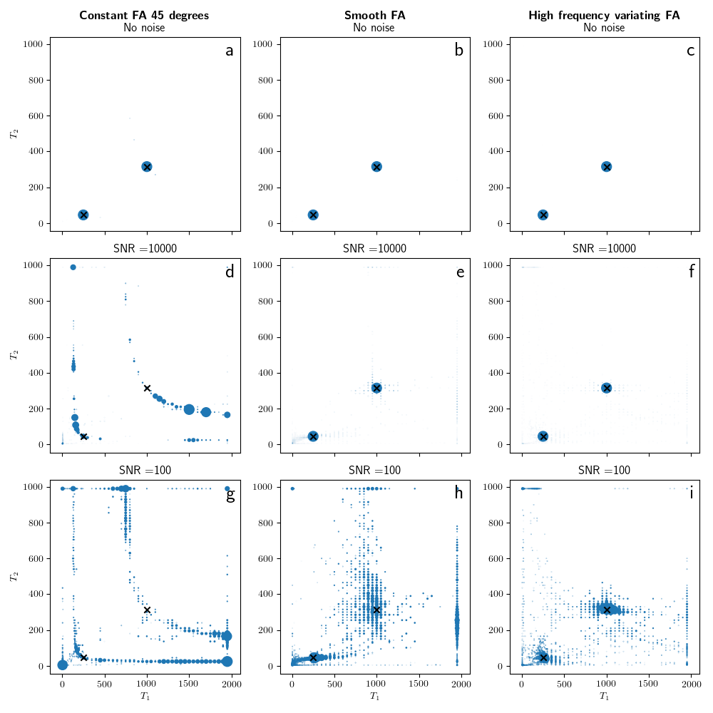
Fig.4 shows an example of the distribution of the matched components in the multi-component matching for the sequences, omitting sequence 2. The multi-component matching is exact for noiseless signals (Fig.4a,b,c). With SNR=10000 sequences 3 and 4 (Fig.4e,f) find some extra components, all with weights below 1%. For SNR=100 (Fig.4g,h) the matched components are spread around the true values but still give an accurate decomposition. For SNR = 10000 the IRbSSFP sequence returns more than 2 large (>10%) components per signal, spread over the corresponding $$$T_1^*$$$-contour lines, which are shown in Fig.5. The matched components can still separate tissues with different $$$T_1^*$$$, but cannot return the corresponding T₁ and T₂ values for the individual components.

The variation in the flip angle breaks the relationship in Eq.1, making it easier to distinguish different T₁ and T₂ combinations. The results in Fig.4 are reproducible for mixtures of different components and varying weights.

Conclusion

Acknowledgements

References

[1] D. Ma et al., “Magnetic resonance fingerprinting,” Nature, vol. 495, no. 7440, pp. 187–192, Mar. 2013.

[2] P. Schmitt et al., “Inversion recovery TrueFISP: Quantification of T1,T2, and spin density,” Magn. Reson. Med., vol. 51, no. 4, pp. 661–667, Apr. 2004.

[3] J. Pfister, M. Blaimer, P. M. Jakob, and F. A. Breuer, “Simultaneous T1/T2 measurements in combination with PCA-SENSE reconstruction (T1* shuffling) and multicomponent analysis,” in Proc. Intl. Soc. Mag. Reson. Med. 25, 2017, p. 0452.

[4] D. McGivney et al., “Bayesian estimation of multicomponent relaxation parameters in magnetic resonance fingerprinting: Bayesian MRF,” Magn. Reson. Med., Nov. 2017.

[5] S. Tang et al., “Multicompartment magnetic resonance fingerprinting,” Inverse Probl., vol. 34, no. 9, p. 094005, Sep. 2018.

[6] C. L. Lawson and R. J. Hanson, Solving least squares problems. SIAM, 1974.

[7] A. M. Bruckstein, M. Elad, and M. Zibulevsky, “Sparse non-negative solution of a linear system of equations is unique,” 2008, pp. 762–767.