4521
Restoring Rotation Invariance of Diffusion MRI Estimators in the Presence of Missing or Corrupted Measurements1Linkoping University, Linkoping, Sweden, 2Brigham and Women's Hospital, Harvard Medical School, Boston, MA, United States
Synopsis
A natural requirement of estimated tissue microstructure features is that they are rotation invariant. So far, the strategy to attain rotation invariance has been to measure in as many uniformly distributed directions as can be afforded and simply compute the projections on an appropriate set of angular basis functions. However, in the presence of missing samples, this approach is sub-optimal. We show that attaching carefully chosen weights to each measurement can achieve a significantly improved rotation invariance, even in the presence of corruptions that break the isotropic sampling symmetry.
Purpose
In many clinical acquisitions, some measurements are corrupted or simply not obtainable, due to, for example, subject motion [RR1 RR2]. We demonstrate that, by introducing measurement weights, an improved precision and rotation invariance of tissue microstructure features can be obtained. We show that optimal measurement weights can be found for any single shell encoding scheme, [RR3], in the presence of missing or corrupted measurements.Methods
Studying anisotropic tissue features, [RR4-RR10], a natural approach is to express the directional dependence as a function on the surface of a sphere using spherical harmonics (SPHs) as a basis. A major advantage using SPHs is that they provide an orthonormal basis on the sphere. A continuous signal, $$$f(x)$$$, can then be represented as:$$c_{nk} = \int{b_{nk}(x)\: f(x)}\: dx~~~~~~~~~~~~{\rm or~(using ~a~single~index)}~~~~~~~~~~~~c_{m}=\int{b_{m}(x)\: f(x)}\: dx$$ where $$$n$$$ is the spherical harmonics degree, $$$k$$$ indicates the order and $$$x$$$ is a vector on the unit sphere. There is a direct relationship between a spherical harmonics representation and a tensor representation [RR11]. All components of an order 2N diffusion tensor can be expressed as a linear combination of spherical harmonics components of degrees 0,2...2N. This implies that all tensor invariants, e.g. eigenvalues, can be found directly from spherical harmonics components. To ensure that the estimates are invariants it is crucial that the computed coefficients correspond to SPH coefficients [RR12]. This requirement is easily violated in the presence of missing data but can be remedied by a simple weighting scheme. All SPHs are basis functions of equal merit and for the purpose of the analysis below the single index expression to the right above is more appropriate.Let $$$y_i$$$ be the set of unit vectors specifying the measured directions and $$$a_i$$$ the weight attached to the corresponding measurement. The spherical harmonics components, $$$c_{m}$$$, of the weighted sampling pattern is then given by: $$c_{m} = \sum_i{b_{m}(y_i)\;a_{mi}}$$ Optimal sets of weights $$$a_{mi}$$$ are readily found by solving the following least squares problem [RR13-RR15], here expressed in matrix notation: $${\bf a}_m=\text{argmin}[\,({\bf B}{\bf a}-{\bf c}_m)^T{\bf W(B}{\bf a}-{\bf c}_m)\,]=({\bf B}^T {\bf W B})^{-1}({\bf W B})^T{\bf c}_m$$ where $$${\bf a}_m$$$ is a vector holding the optimal weights for the $$$m$$$th SPH. $$${\bf B}$$$ is a matrix containing the values of the spherical harmonics basis sampled at the orientations given by $$$y_i$$$. $$${\bf W}$$$ is a diagonal matrix that contains the weight attached to a goodness of fit for each spherical component. As a 'rule of thumb' $$${\bf W}$$$ can be chosen as the expected signal energy for each SPH basis function. $$${\bf c}_m$$$ is the ideal response vector for the $$$m$$$th SPH.
Results
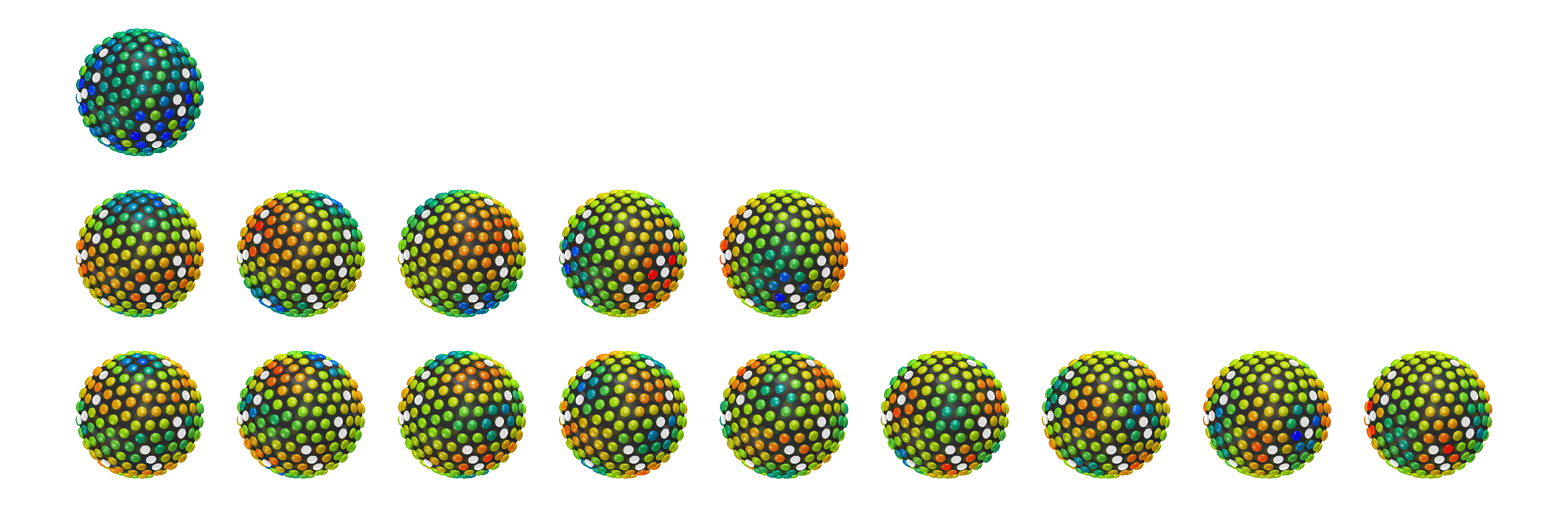
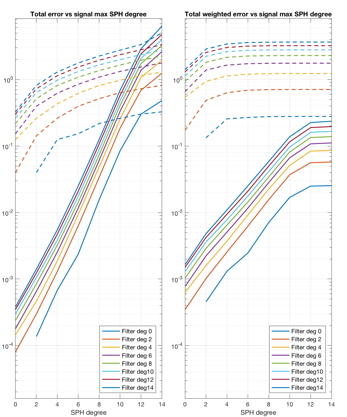
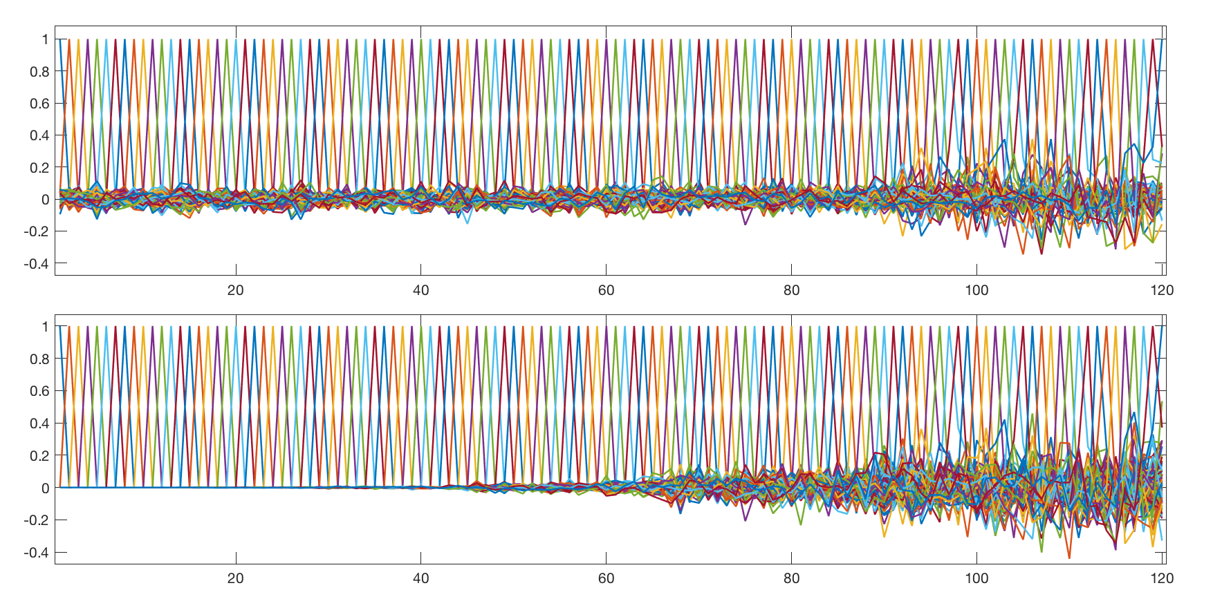
Two cases are presented: Acquisition in 21 orientations with 2 measurements lost (figures1 and 2) and acquisition in 120 orientations with 12 measurements lost (figures 3-5). Figures 1 and 3 show the distribution of the optimal weights, $$${\bf a}_m$$$, for the first 15 SPH basis functions (orders 0, 2 and 4). Figures 2, 4 and 5 show how much signal is picked up from other than the intended basis function in two different ways.Figure 5 shows the 'spectrum' of the SPH component estimators. Ideally no other signal components should be picked up. The curves in figures 2 and 4 can be seen as an error that will destroy invariance properties of SPH based estimates. The error depends both on the SPH degree that is measured (different curves) and the maximum SPH degree of the signal being measured (x-axis). For low b-values the signal will only contain low SPH degrees but for high b-values much higher degrees may be present. For a reasonable signal SPH content (the W weighted case) the reduction in the invariance corrupting errors are in the order of 10 to 100 times. This provides a strong indication that employing optimal weighting yields a significantly improved rotational invariance in the case of lost measurements.
Discussion and Conclusion
We have demonstrated a straightforward scheme for optimizing the weighting of directions when analysing microstructure anisotropy. The main limitation of this study is that we have not investigated if weighting yields a relevant benefit in actual data, since the effects of rotational variance may be small compared to other sources of variance and bias, such as measurement noise. On the other hand the cost of using our optimized weighting scheme is negligible and it can be applied to any existing directional protocol. In conclusion, we have provided a method for optimal weighting of signals for maintaining the rotation invariance of the estimates in the presence of corrupted data.Acknowledgements
The authors acknowledges the following grants:The Swedish Research Council 2015-05356, the Swedish Foundation forStrategic Research AM13-0090, the Linneaus center 'CADICS' and the Knut and Alice Wallenberg foundation 'Seeing Organ Function'.References
[RR1] C. Guan Koay, S. A. Hurley, and M. E. Meyerand, Medical Physics (2011)
[RR2] P. A. Cook, M. Symms, P. A. Boulby and D. C. Alexander, Magn. Reson. Imaging, 25:1051–1058 (2007)
[RR3] D. Jones et al., Magn. Reson. Med. 42 (3), 515-525 (1999)
[RR4] F. Szczepankiewicz et al., Neuroimage 104, 241-252 (2015)
[RR5] M. Lawrenz and J. Finsterbusch, Magn. Reson. Med. 73 (2), 773-783 (2015)
[RR6] S. Jespersen et al., NMR Biomed. 26 (12), 1647-1662 (2013)
[RR7] E.T. McKinnon et al., Magn. Reson. Imaging (2016)
[RR8] F. Szczepankiewicz et al., Proc. Intl. Soc. Mag. Reson. Med. 24, 2065 (2016)
[RR9] A. Leemans, Proc. Intl. Soc. Mag. Reson. Med., 2009
[RR10] E. L. Altschuler et al., Phys. Rev. Lett. 78 (1997)
[RR11] E. Özarslan and T.H. Mareci, Mag. Reson. Med. Volume50 955-965 (2003)
[RR12] M. Kazhdan, T. Funkhouser, and S. Rusinkiewicz Eurographics Geom. Proc. (2003)
[RR13] F. Szczepankiewicz, C-F. Westin and H. Knutsson, Proc. Intl. Soc. Mag. Reson. Med. Honolulu, Volume: 25 (2017)
[RR14] H. Knutsson and C-F Westin, CVPR'93 New York City 515-523 (1993)
[RR15] H. Knutsson et al., Proc. 11th Scan. Conf. on Image Analysis: Greenland, 185-193. (1999)
Figures
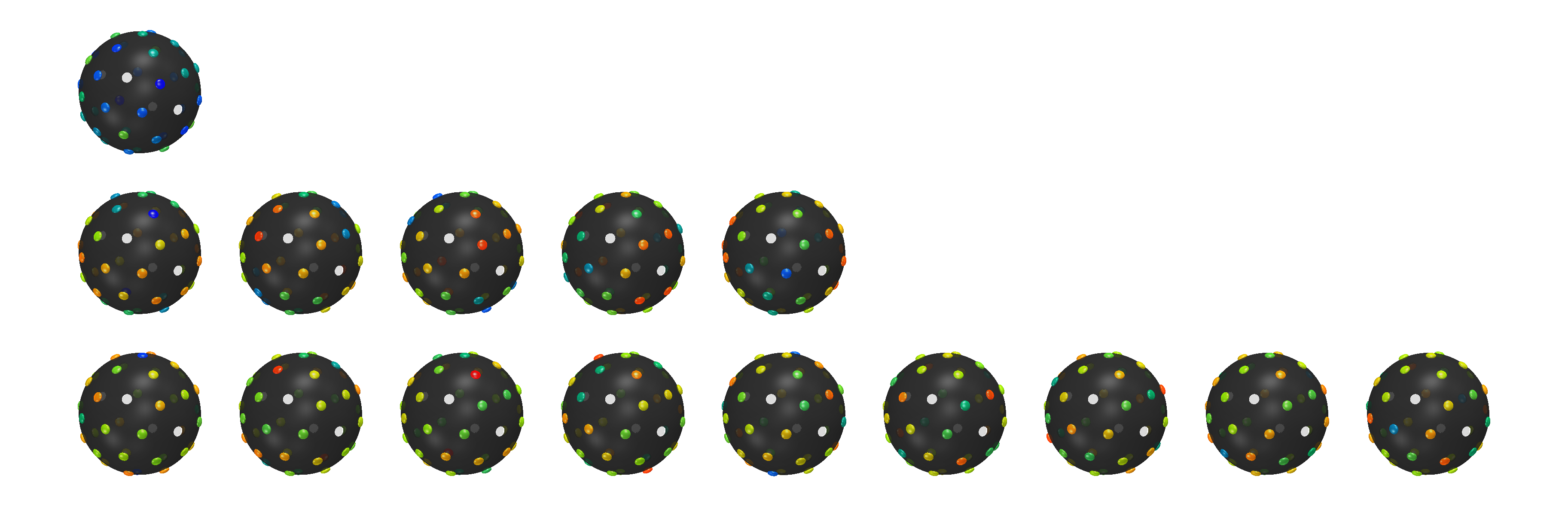
The figure shows the result of the weight optimization for the case of 21 uniformly distributed orientations (42 diametrically positioned points) with two missing measurements. Starting at the top the rows show results for spherical harmonic degrees 0, 2 and 4. Colors indicate filter weight values, blue is most positive and red is most negative. The missing measurement locations are shown in white. The top plot shows the weights for the zero degree spherical harmonics. For a complete uncorrupted acquisition all weights would be identical. It is clearly visible how the weights around the missing measurements are increased in order to compensate for the loss.
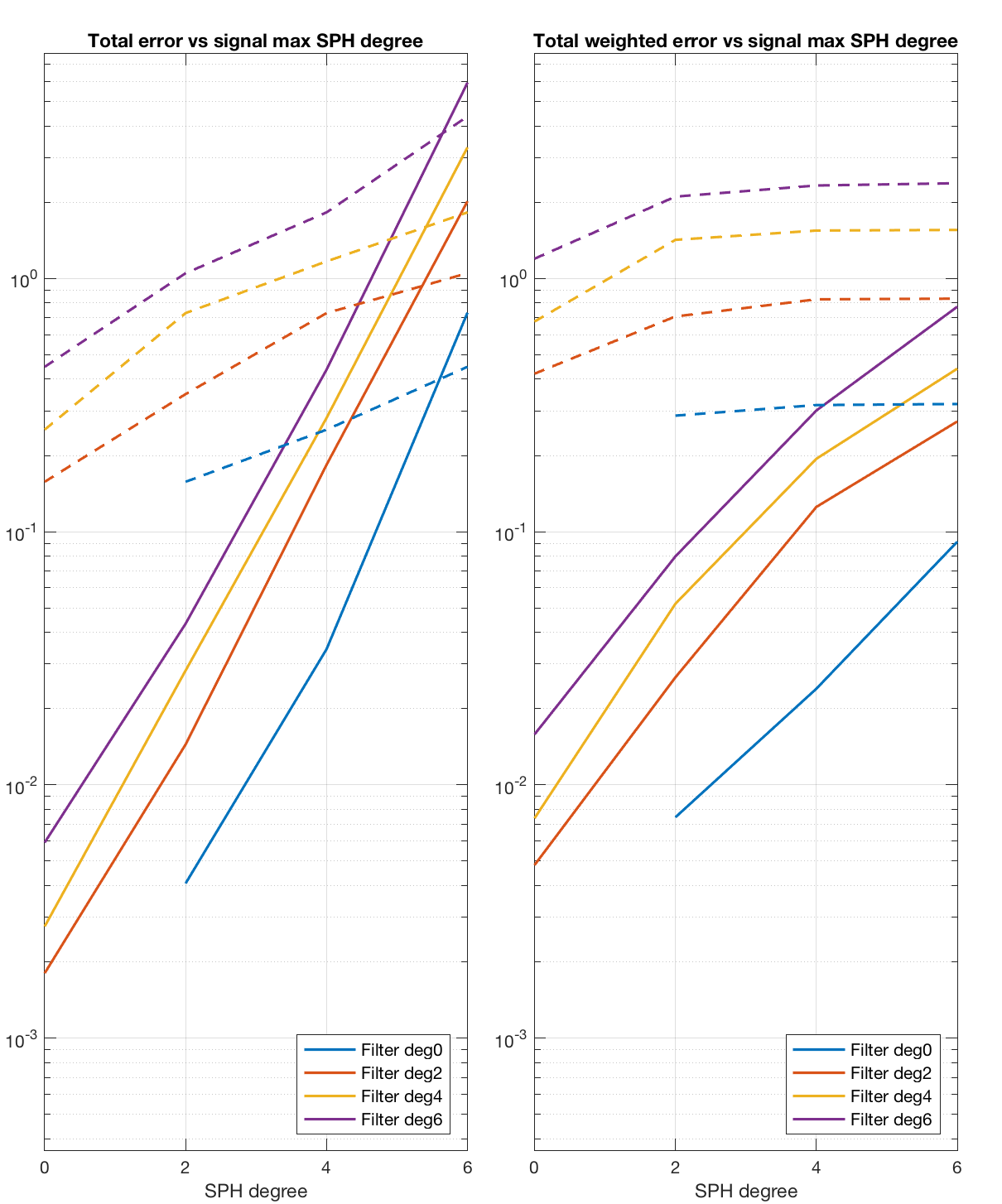
Estimated error distribution for the case of 21 uniformly distributed orientations with two missing measurements. The error is given as a function of the signals maximum spherical harmonic degree and the degree of the estimated SPH basis function. The left plot shows the result for a signal with equal energy for all spherical harmonics up to the degree indicated on the x-axis. The right plot shows the result where the energy decreases as specified by $$$W$$$. The dashed lines show the errors using unaltered spherical harmonic function values. The continuous lines show the marked decrease of the errors using the optimized weights.