4507
Investigation of the Cost Function for Joint Estimation of Object and B01University of Zurich and ETH Zurich, Zurich, Switzerland
Synopsis
Due to their short read-out time single-shot techniques are frequently used for several imaging modalities but they are prone to static B0 off-resonance artifacts. To avoid separately acquired field maps joint estimation of the object and the B0 map has been proposed as a potential solution alternating between updating an object and a field map guess. A measure to compare cost functions is introduced and two different joint estimation cost functions are investigated whereby a new cost function in image space is suggested. It shows its potential if only a less reliable B0 map guess is given.
Introduction
Single-shot techniques are the underlying workhorse for several imaging modalities such as fMRI but due to their comparably low bandwidth they are particularly sensitive to magnetic field inhomogeneities. A particular attractive implementation is to jointly estimate (JE) a field map and the object as it does not require separate B0 map acquisition and can adopt to changes in B0 during the course of the acquisition. A previously implemented approach is to minimize a regularized least squares problem in k-space [1] where the object and the field map guess are updated in alternating fashion. A crucial problem of this approach is the non-convexity of the cost function. In this work we aim to assess the non-convexity of the cost function and suggest an alternative cost function showing hope for greater attractor sizes towards the global minimum. In particular the dependence on the starting point of the optimization is analyzed employing gradient descent.Methods
Cost function in k-space
A previous implementation [1] proposed to minimize the following least-squares problem on the signal data $$$s(t)$$$
$$L(\omega_0(x),o(x))=\left\lVert s(t)-E(k(t),\omega_0(x))\,\cdot\,o(x)\right\rVert^2$$
$$\hat{\omega}_0(x),\hat{o}(x)=\text{argmin}\;L(\omega_0(x),o(x))$$
where $$$k(t)$$$ describes the k-space coordinate, $$$o(x)$$$ the imaged object, and $$$E$$$ the encoding matrix with entries
$$E_{mn}=\exp(-i\omega_0(x_n)t_m)\exp(-i2\pi k(t_m)\cdot x_n)$$.
One reason for the non-convexity of the problem are phase wraps of the complex signal.
Magnitude cost function in image space
Another cost function is proposed based on the fact that the magnitude of the point spread function (PSF) of EPI and spiral trajectories is a one to one mapping for different field offsets $$$\omega_0(x)$$$:
$$L(\omega_0(x), o(x)) = \left\lVert \mid E^+(k(t),0)\cdot s(t)\mid - \mid E^+(k(t),0)\cdot E(k(t), \omega_0(x)) \cdot o(x)\mid\right\rVert^2$$
$$\hat{\omega}_0(x), \hat{o}(x) = \text{argmin}\;L(\omega_0(x), o(x))$$
Here, $$$E^+$$$ describes the pseudo-inverse of the operator $$$E$$$. The considered images are in the distorted space as the $$$E^+$$$ operator is computed for $$$\omega_0(x) = 0$$$.
Gradient Descent and Attractor Size
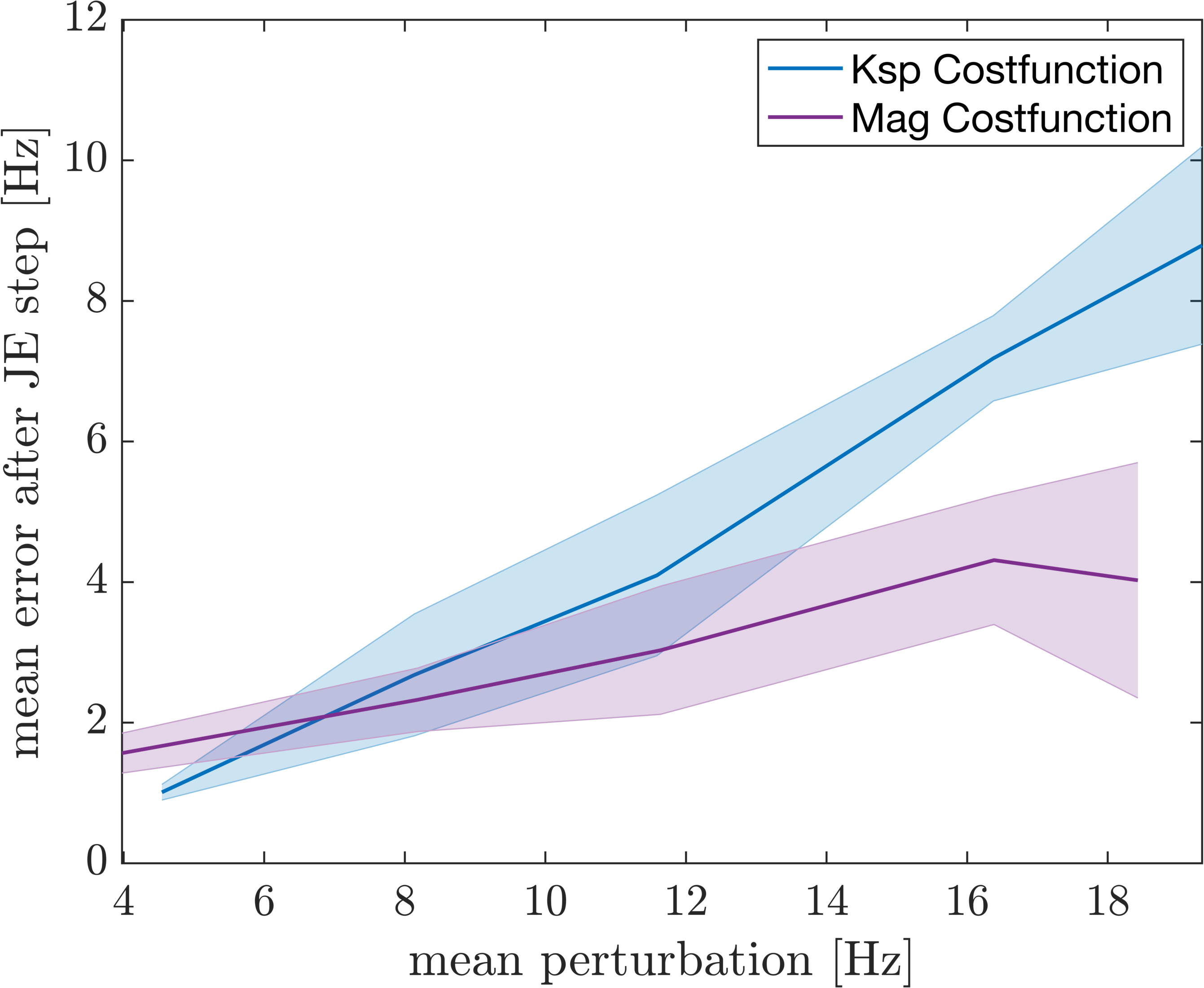
A quality measure of a cost function can be defined by the attractor size defined as the maximum disturbance of the point of interest from which a gradient descent still converges to (or close to) the point of interest. To assess the performance of the cost function attractor sizes were evaluated by differing the quality of the initial guess and a gradient descent algorithm was used to perform the B0 optimization of the JE problem (Fig. 1).
Measurement parameters and B0 fitting
MR scanning was performed on a 3T MR system (Philips Healthcare, Best, The Netherlands) using an 8-channel head coil array equipped with 16 magnetic field sensors (Skope MR Technologies, Zurich, Switzerland) [2] to record the actual k-space trajectory. A spiral in/out sequence with TE: 43 ms, FOV: 22 cm, resolution: 1x1 mm was played out. An initial field map guess was obtained by splitting the acquired data into two images and fitting the image phase. For reference, a field map was fitted from a 2-echo gradient echo (GRE) sequence.
Results
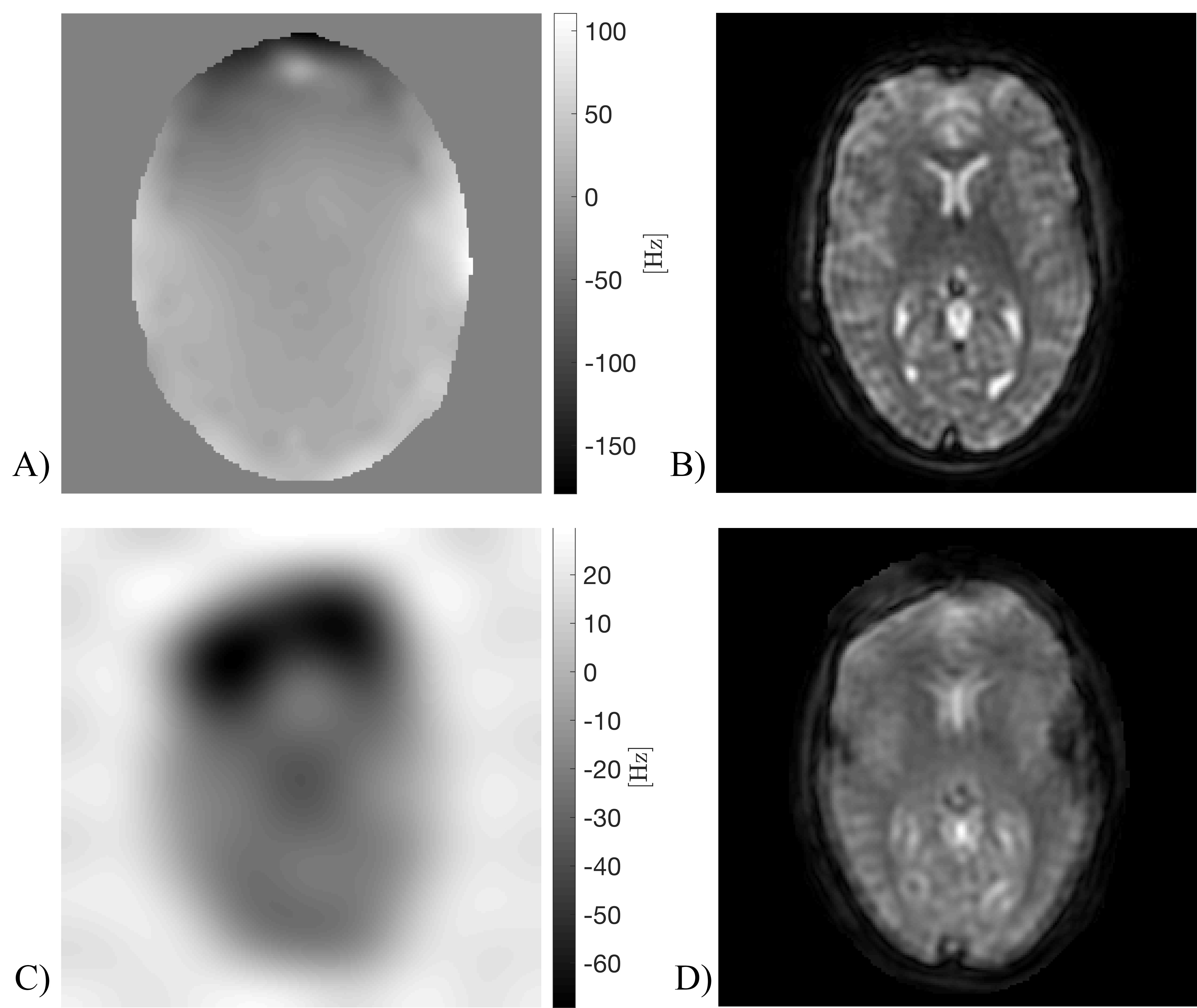
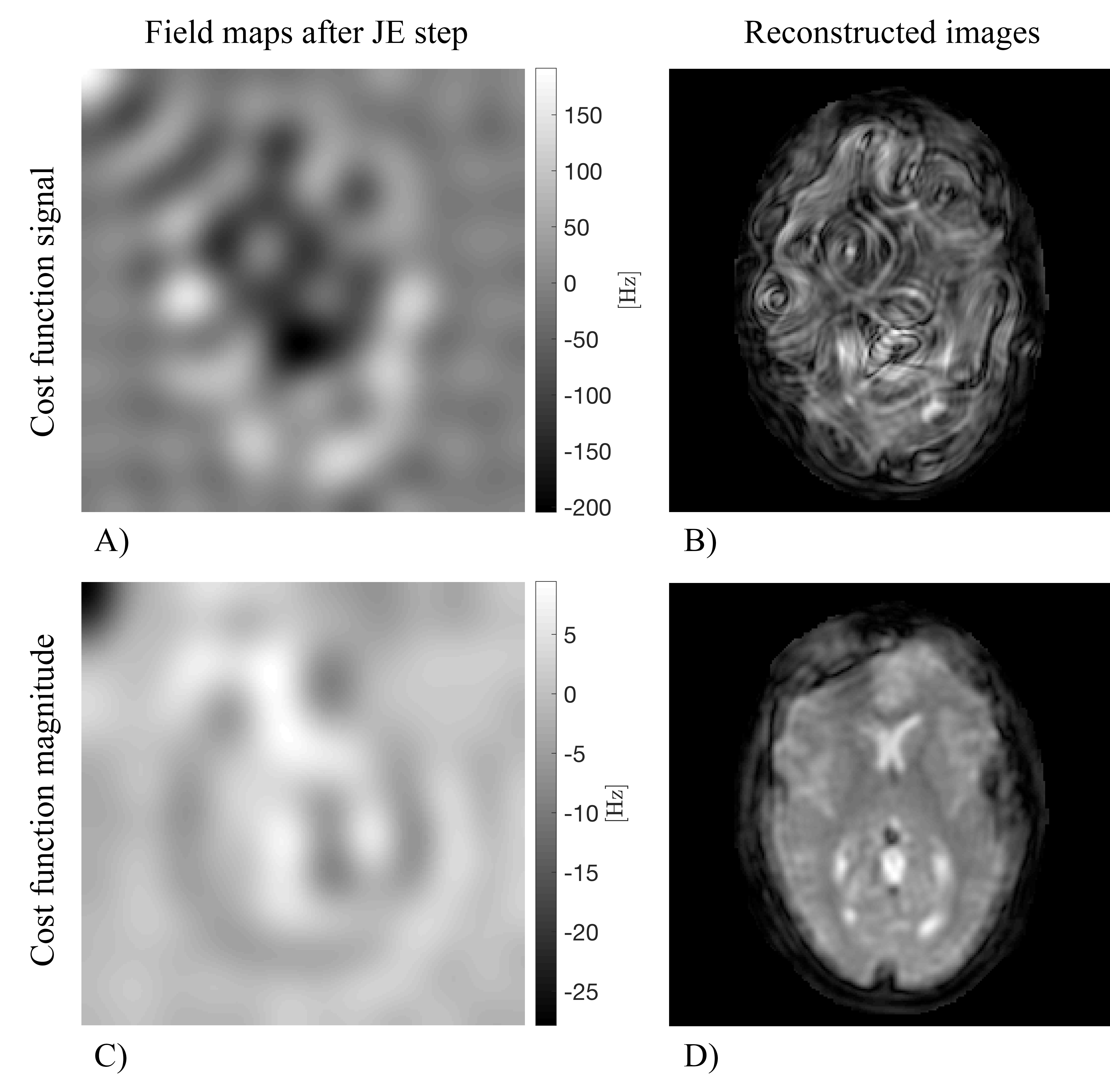
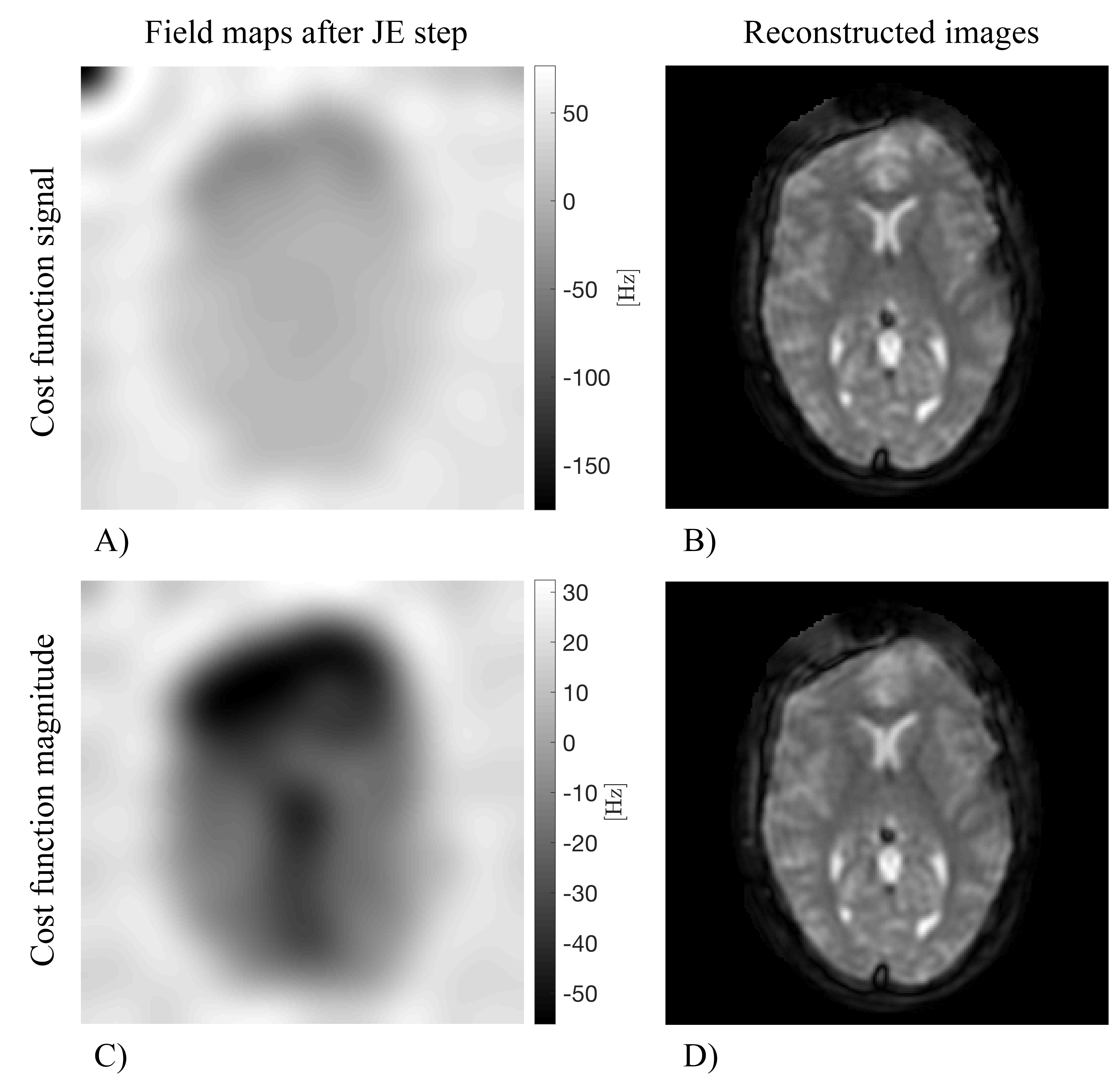
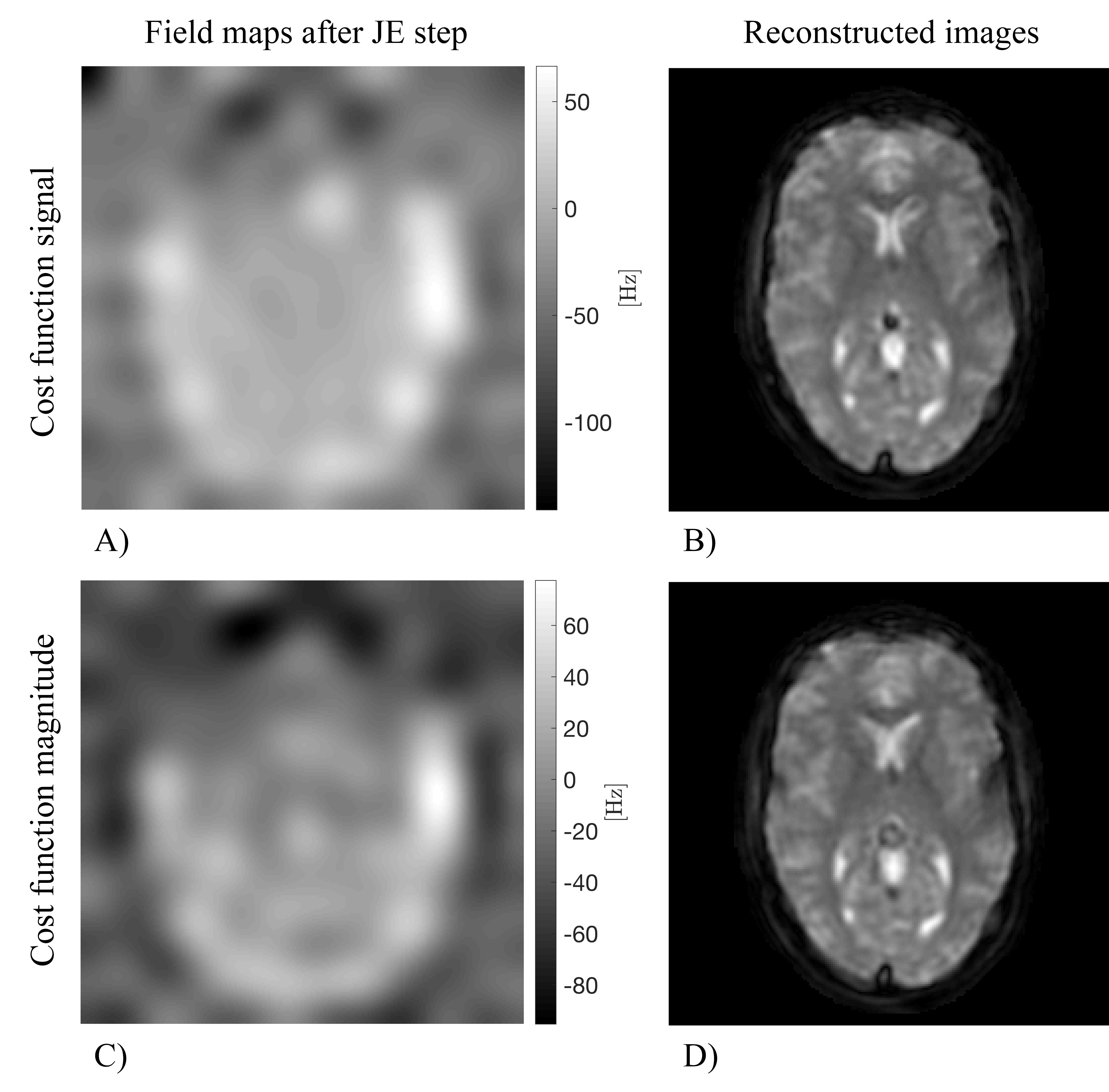
To allow a comparison of the different scenarios in-vivo a fixed object guess (Fig. 2B) was used, reconstructing the signal using the GRE field map (Fig. 2A) [3]. The result of the JE algorithm depends on the initial field map guess, which can be obtained from: (1) a zero field map; (2) a field-map fitted from two distorted images (if $$$s(t)$$$ permits reconstructing two images with temporal information); (3) a previously measured field-map. The field maps as well as the reconstructed images using a constant field map of 0 Hz as initial guess differ a lot for the two cost functions (Fig. 3). Less deviation is visible using a distorted field map (Fig. 2C) as initial guess for both cost functions (Fig. 4). Nevertheless, the reconstructed objects still show some distortions. In the case of small perturbation of the GRE field map (Fig. 2A) a map close to the initial map could be found by either of the cost functions. These findings are in accordance with the simulation data (Fig. 2).Discussion and Conclusion
The attractor size of the proposed magnitude cost function was found to be larger compared to the k-space cost function. The findings could be substantiated with an in-vivo example. The larger attractor size for an initial guess with a greater mean deviation suggests to use the magnitude cost function if no reliable initial guess of the field map is available. Following the results, a possible strategy might be to start with the magnitude cost function and switch after some iterations to the k-space cost function as its evaluation is computationally less expensive. The results of this study show that a different cost function can increase the attractor size of the non-convex B0 optimization included in the JE algorithm and hence make JE more robust.Acknowledgements
No acknowledgement found.References
[1] Sutton et al. – Dynamic Field Map Estimation Using a Spiral-In / Spiral-Out Acquisition
[2] Kennedy et al. – An industrial design solution for integrating NMR magnetic field sensors into an MRI scanner
[3] Barmet et al. - Sensitivity encoding and B0 inhomogeneity - A simultaneous reconstruction approach, Proceedings of the ISMRM 2005
Figures