4498
Minimal Linear Networks for MR Image Reconstruction1Faculty of Psychology and Neuroscience, Maastricht University, Maastricht, Netherlands
Synopsis
We propose minimal linear networks (MLN) for MR image reconstruction that employ complex-valued, axis-dependent and fully- and neighborhood-connected layers with shared and independent weights, Their topology is restricted to the minimum required by the MR-physics, without nonlinear activation layers. The suggested MLN perform well in reconstructing imaging data acquired under challenging real-world imaging conditions, specifically an Arterial Spin Labeling perfusion experiment with spiral sampling at 7 Tesla. Despite the strong B0 field inhomogeneities at 7T, artifact-free images are obtained that are capable of resolving the minute perfusion signal changes. The results show that even without nonlinear activation and higher-order image manifold description as used by others, deep-learning algorithms and framework, and learning from large realistic datasets, can play a significant role in the success of image reconstruction.
Introduction
Deep learning (DL) techniques have been shown to have great potential of outperforming compressed sensing and other advanced approaches to MR image reconstruction. In order to probe into the elements that contribute to the recent successes of DL, we develop a minimal “neural” network (MLN) for MR image reconstruction, without any non-linearity (e.g. relu, etc), with no bias variables, and all layers operating on the complex-valued data. The method is demonstrated on 7T ASL perfusion measurements using spiral acquisitions which are particularly sensitive to B0 field inhomogeneity, and benchmark multi-channel undersampled 2D Cartesian data.Methods
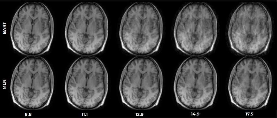
We designed MLN architectures and applied them to n two scenarios in MR reconstruction: (i) undersampled non-Cartesian 7T spiral acquisitions with 32-channels, including correction for B0 field inhomogeneity, and (ii) highly undersampled Cartesian 8-channel data with Poisson-disk sampling. Fig. 1A introduces the subspace fully-connected (SFC) layer: fully-connected on some axes, with weight sharing on some axes and independent weights on the others. We denote it by [ Independent axes | Shared axes | FC axes: old -> new ]. The suggested network operates on regridded data (Fig. 1B), following these steps for time-segmented B0 field inhomogeneity correction1 : for each k-space location (including missing points), the data from the neighboring nNeighbors=12 sampled k-space locations, and from all channels, is concatenated, resulting in a 3D matrix of the form kROxkPExnNeighbors⋅nChannels for each training dataset. The network first applies a k-space pointwise independent kernel operation: [kRO,kPE | - | nNeighbors*nChannels -> nTS] to nTS=7 “time-segments”, followed by FT along RO and PE: [ - | kRO, TS| kPE->PE], [ - | PE,TS | kRO->RO], and finally a “maps” operation to combine the reconstructed images from the different “time-segments / compressed channels” into the final image: [RO,PE | - | nTS -> 1]. The network was trained on 10,000 images, randomly extracted from the Human Connectome Project 2 database, with random synthesized phase, flipping, 90o rotation and cropping. Actual MRI data from N=4 subjects was obtained on a 7T scanner with 32-channel head coil, using a 2D spiral perfusion sequence. Each spiral readout was 12.5ms long with 5120 samples (FOV 192mm, in-plane resolution ~1.7mm, slice thickness 3mm, arterial spin labeling preparation as described in 3 : 80 repetitions; 4 min). For reference, images were also reconstructed using BART 4 and L1-CG-ESPIRIT 5 with gpuNUFFT 6 and time-segmented B0 correction 1. For the experiments in (i), undersampling ratios of ~8.8, 12.9 and 17.5 we applied, and resulting image quality evaluated using the SSIM metric. The MLN was implemented in TensorFlow, with Adam optimizer, 0.002 learning rate, and overall standard settings.Results
Fig. 2 presents 7T spiral results obtained using various MLN topologies. The single-”time”-segment topology does not compensate for B0 inhomogeneities, resulting in blurring and artifacts. Similarly, the topology with shared weights on the k-side t resulted in a blurry reconstruction, while the topology with independent localized k-side kernels and 7 time segments resulted in a nearly artefact free image. Using >7 time-segments did not further improve the image quality. Fig. 3 shows a zoomed view of a single slice, for the reference ESPIRiT reconstruction with image-to-signal model to which we added time-segmented B0-correction. The MLN produces a clean artifact-free image. This is further evidenced in the multi-slice reconstruction of the ASL perfusion experiment shown in Fig. 4. While producing sharp individual images, the MLN did retain the temporal changes, allowing for extraction of the minute ~1% perfusion signal changes (Fig. 4E). The results were consistent across all participants. Finally, the MLN was tested in a benchmark settings, highly undersampled 8-channel Cartesian data. Figure 5. Shows MLN results on a representative image vs. reference reconstruction techniques (data not shown). The simple architecture makes the weights more interpretable, and consisted of k-side regridding kernels and image-domain combination maps into the final image (not shown). Monte-Carlo and pseudo replica reconstructions of real data showed slightly higher noise amplification for MLN than in the other techniques, attributable to the absence of a denoiser or denoiser-like elements such as image-based regularization.
Discussion and Conclusion
Neural networks are a very strong tool that can outperform traditional reconstruction techniques even when simplified to the minimum. The proposed MLN have very weak descriptive power, and do not use non-linear “neurons” , excluding “manifold” explanations. The trained weights have high interpretability, corresponding to traditional reconstruction steps. We conjecture that describing the signal-image relationship under specific transformations is easier and more validatable than describing the domain/manifold of MR images, were most effort has been put.Acknowledgements
This project was funded by NWO 016.VIDI 178.052 to B.A.P. Data was acquired at Scannexus BV, Maastricht, NL (www.scannexus.nl). The authors thankfully acknowledge the help of Dr. Dimo Ivanov with the ASL data acquisition and analysis, as well as Sriranga Kashyap for assistance with perfusion analysis and preparing the figures..References
1. Sutton BP, Noll DC, Fessler JA. Fast, iterative image reconstruction for MRI in the presence of field inhomogeneities. IEEE transactions on medical imaging 2003.
2. Van Essen DC, Smith SM, Barch DM, Behrens TEJ, Yacoub E, Ugurbil K, WU-Minn HCP Consortium. The WU-Minn Human Connectome Project: an overview. Neuroimage 2013;80:62–79. doi: 10.1016/j.neuroimage.2013.05.041.
3. Ivanov D, Poser BA, Huber L, Pfeuffer J, Uludağ K. Optimization of simultaneous multislice EPI for concurrent functional perfusion and BOLD signal measurements at 7T. Magn. Reson. Med. 2017;78:121–129. doi: 10.1002/mrm.26351.
4. Uecker M, Tamir J, Ong F, Holme C, Lustig M. BART: version 0.4.01. 2017.
5. Uecker M, Lai P, Murphy MJ, Virtue P, Elad M, Pauly JM, Vasanawala SS, Lustig M. ESPIRiT--an eigenvalue approach to autocalibrating parallel MRI: where SENSE meets GRAPPA. Magn. Reson. Med. 2014;71:990–1001. doi: 10.1002/mrm.24751.
6. Knoll F, Schwarzl A, Diwoky C. gpuNUFFT-an open source GPU library for 3D regridding with direct Matlab interface. Proc. ISMRM 2014.
Figures
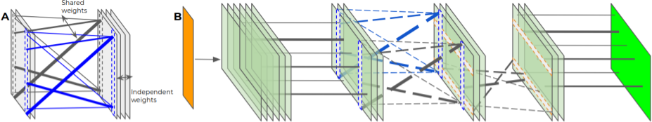
Figure 1: A. Subspace fully-connected (SFC) layer. B. Network topology mimicking the time-segmented B0 inhomogeneity corrected signal->image pipeline.
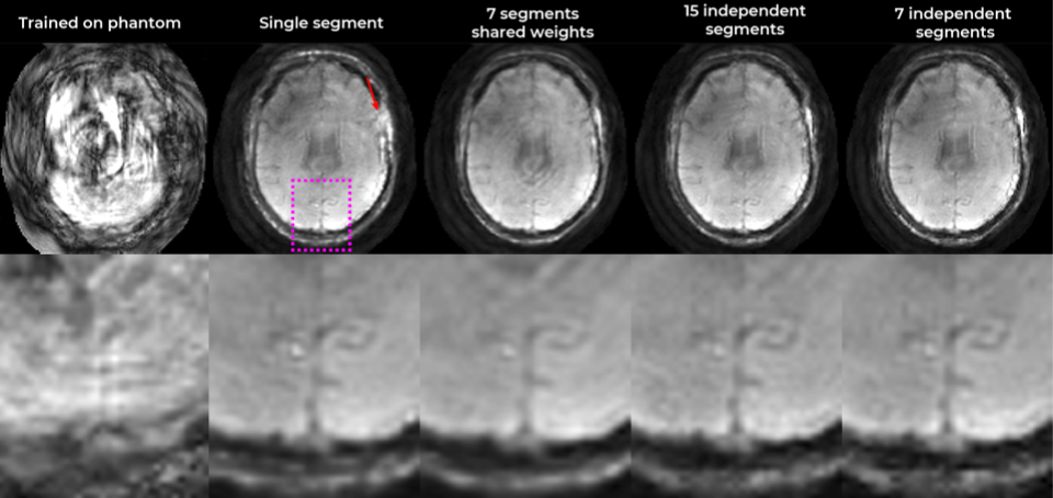
Figure 2: Results obtained using different network topologies, on real data. Leftmost: result obtained when using random phantom images (multi-ellipses) as training. In that case, the network did reconstruct other multi-ellipses instances (not shown), but did not generalize to real data.
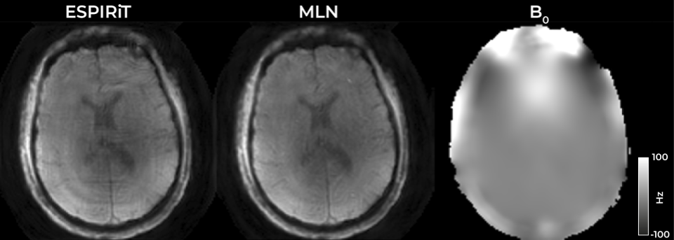
Figure 3: Comparison with reference reconstruction, adapted with time-segmented B0-field inhomogeneities corrected image-to-signal model. Rightmost: The B0 field estimation obtained from multi-echo GRE .
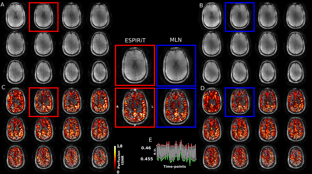
Figure 4: Results on multiple slices using reference method (A) and MLN (B), and corresponding perfusion maps (C,D) obtained from reconstructed time-series. Center: zoomed-up version. The MLN reconstruction is cleaner, which also resulted in artifact-free perfusion map. (E) Time course (averaged over perfused voxels) showing the reconstruction was sensitive to the minute signal changes, due to perfusion, preserving the expected 1% in signal change.