4441
Prospective motion correction for compressed sensing 3D TSE sequence1Dept. of Radiology, Medical Physics, Medical Center University of Freiburg, Faculty of Medicine, University of Freiburg, Freiburg, Germany, 2Siemens Healthcare GmbH, Erlangen, Germany
Synopsis
A compressed sensing 3D TSE Sequence prototype (CS-SPACE) was enhanced by prospective motion correction (PMC). For T1-weighted imaging this sequence uses a center-out trajectory along each echo train and sparser sampling with increasing distance from the center. Motion during such echo trains can result in unexpected image artifact behavior. In this work, we investigate whether for a particular echo train structure, a center-out trajectory and compressed sensing PMC can correct for motion artifacts.
Introduction
Imaging examinations for research studies as well as clinical routine
demand for increasingly higher spatial resolutions without increasing scan
times. This can be achieved with modern acquisition strategies such as
compressed sensing (CS) and usage of multiple receive channels (parallel
imaging)1,2.
Recently, a compressed sensing variable flip angle 3D TSE sequence
prototype was introduced (CS-SPACE)4,6, which allows for isotropic
high-resolution imaging and showed potential in particular for imaging of
cerebral vascular structures3.
(Without CS and parallel imaging: 20min. With parallel imaging: 11min.
With CS: 5min)
However, similar to standard 3D TSE sequences, CS-SPACE imaging remains
sensitive to motion. Previous work4 was using navigators to avoid pronounced
motion artifacts by means of discarding and reacquiring echo trains affected by
motion. This work aims to introduce prospective motion correction (PMC) with an
external tracking device5 into the CS-SPACE sequence and presents initial
results in healthy volunteers.Methods
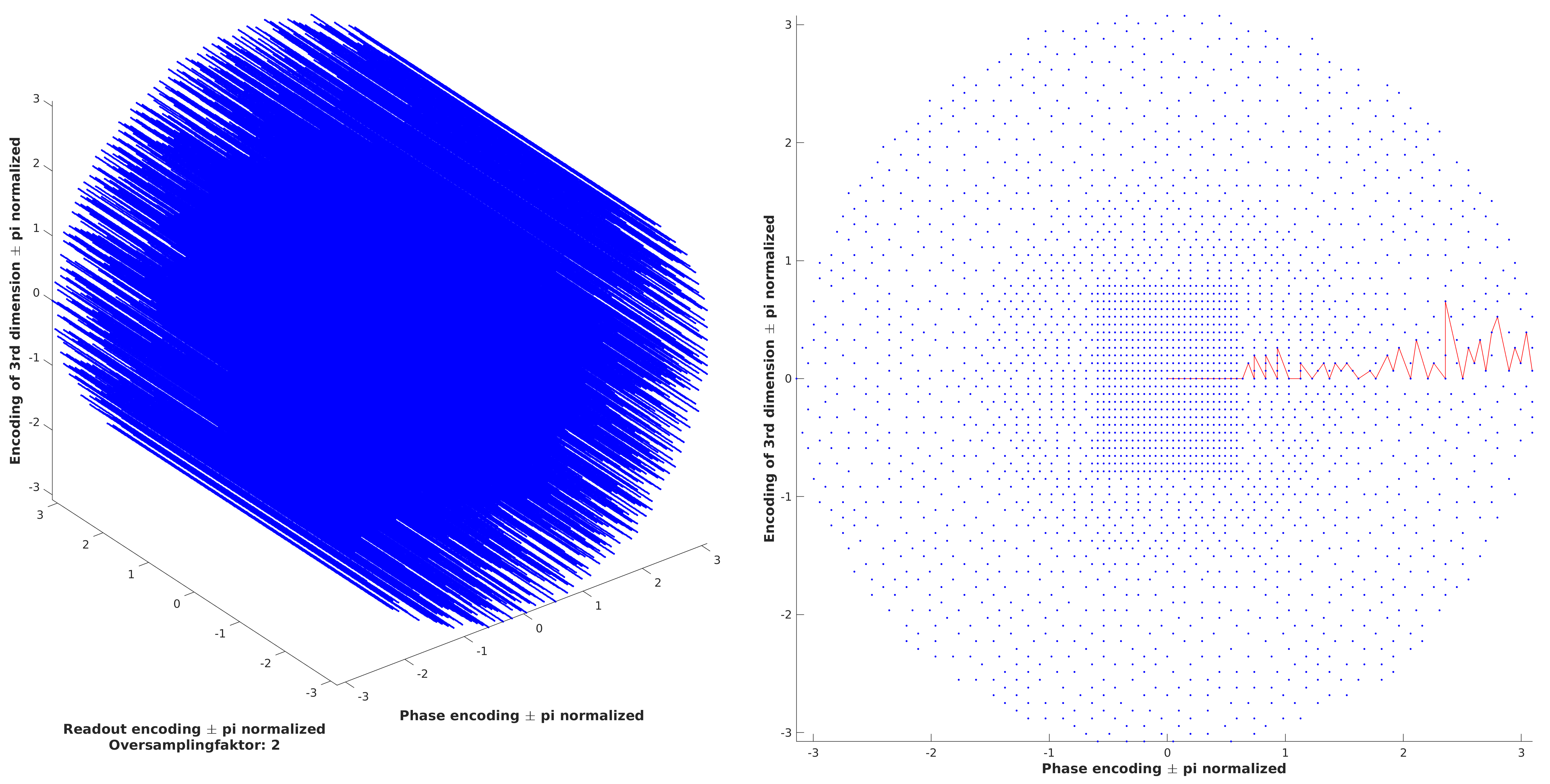
Sequence: The CS-SPACE sequence uses Cartesian k-space sampling together with a pseudo-random Poisson-disc variable density pattern6 (Fig.1). A T1-weighted protocol was used. Therefore, in each TR multiple echoes are sampled in an echo train starting from the fully sampled k-space center and moving towards outer k-space regions between every TE (Fig.1). The sequence was modified to incorporate correction of the slice position once per TR just before the application of the initial excitation RF pulse. TSE sequences with correction per echo are likely to lose signal due to the violation of the CPMG-constraint because of tracking inaccuracies. Due to relatively short echo trains used in T1-wighted imaging and center-out trajectory per echo train, a single correction of the slice position at the beginning of each TR was considered appropriate. Whole-brain measurements were done in sagittal slice orientation with 0.55mm isotropic resolution (384x384x256Voxel), 50 echoes per echo train, TR:800ms, TE:5.1ms, CS-sampling-factor:0.2
Hardware: A MAGNETOM Prisma (Siemens Healthcare, Erlangen, Germany) 3T MRIscanner was used together with the system’s 64-channel head coil. Additionally, a marker based tracking system was used7 to provide the necessary correction motion data. The marker was fixed on a mouthpiece fitted on the upper yaw
Imaging: Experiments were done in three healthy, MR-experienced volunteers under the following conditions: (i) the volunteers’ head was fixed via cushions (reference data set without motion), (ii) the volunteers were instructed to move the head and with motion correction disabled (motion data without correction), and (iii) the volunteers were instructed to move the head as in (ii) but with motion correction activated (motion data with correction).
Reconstruction: Reconstruction of undersampled k-space data was done via a compressed sensing reconstruction with L1 regularization3,6 and 20 iterations.
Results & Discussion
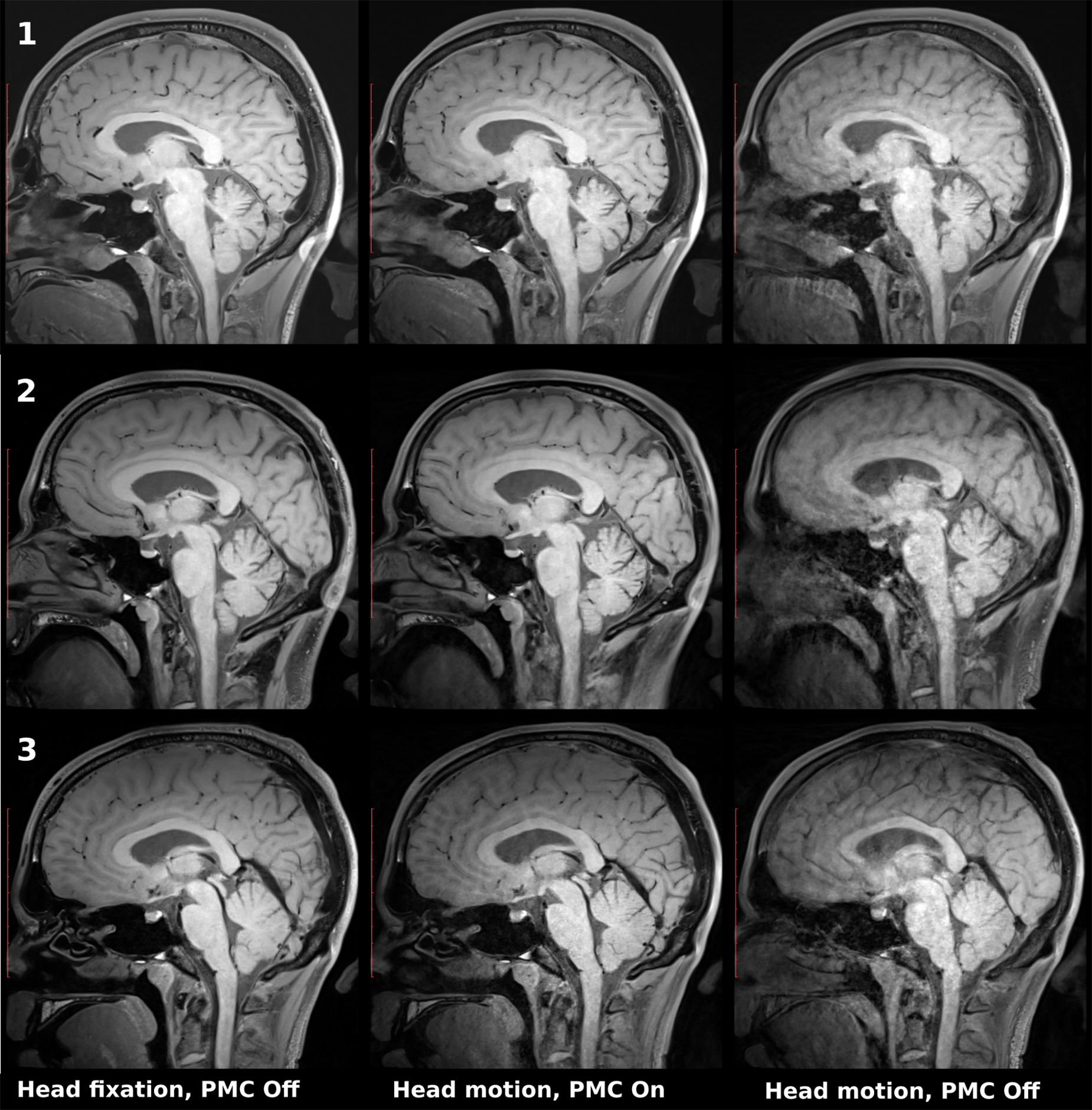
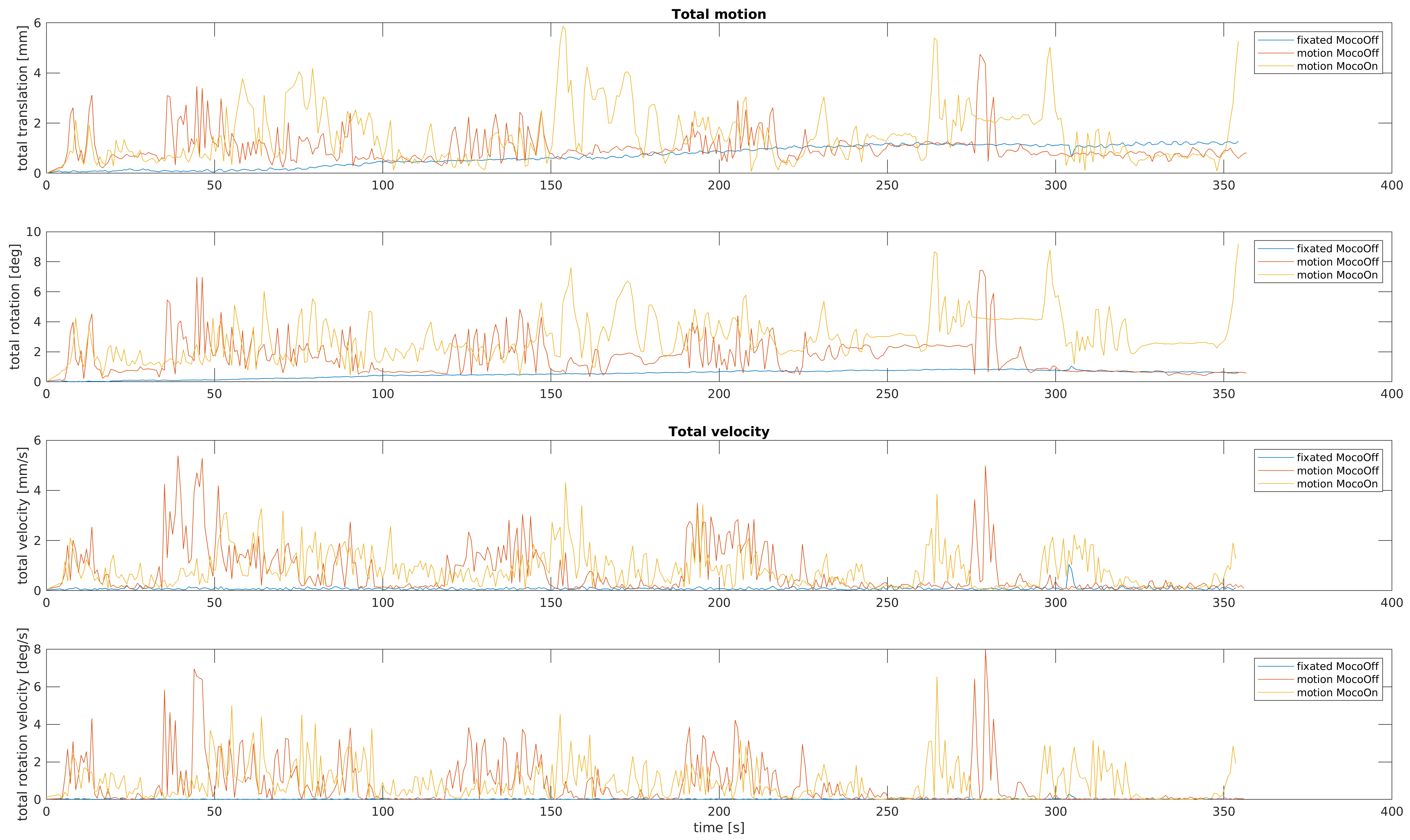
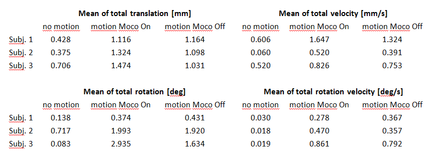
Representative images from the volunteer measurements without motion and the two scans with arbitrary motion are shown in Fig.2. To illustrate that the motion patterns of the subjects were comparable between the two scans with motion, the tracking data for one subject is plotted in Fig.3. Statistical parameters of the translational and rotational motion patterns for all subjects are summarized in Table.1. In the measurements with subject #3, the range of motion was larger than for #1 and #2, so that the marker was partially hidden under the case of the coil. Therefore, in the motion corrected measurement 487 tracking positions were missing (1.63%, usually this is below 0.03%). Compared to the reference images, images acquired with PMC in presence of motion still show subtle shading artifacts (Fig.2). However, motion-corrected images for subjects #1 and #2 exhibit image quality comparable to the reference with head fixation. Only in subject #3, pronounced motion artifacts are visible in the motion-corrected images because the tracking information was partly missing. Nevertheless, the quality of the motion-corrected images is still superior to the non-corrected data. The actual motion patterns of subjects #1 might render the patterns as seen in subjects that feel uncomfortable during the scan. The motion pattern of subject #3 might render scan situations as seen with incompliant or highly uncomfortable subjects. However, in all cases PMC substantially improved image quality so that image quality was still acceptable for further evaluation.Conclusion
Prospective motion correction can improve image quality in CS-SPACE imaging when motion is present. With typical motion patterns, the image quality nearly reaches the quality of reference images. Strong motion and loss of marker tracking degrade image quality notably. The PMC CS-SPACE sequence might be especially interesting for research studies which rely on excellent image quality for example when automated post-processing are applied afterwards for segmentation so that motion artefacts are highly distracting.Acknowledgements
This work is partially funded by NIH grant 2R01DA021146References
1. Lustig M, Donoho D, Pauly JM. Sparse MRI: The application of compressed sensing for rapid MR imaging. Magnetic Resonance in Medicine. 2007;58(6):1182–1195. doi:10.1002/mrm.21391
2. Pruessmann KP, Weiger M, Scheidegger MB, Boesiger P. SENSE: Sensitivity encoding for fast MRI. Magnetic Resonance in Medicine. 1999;42(5):952–962. doi:10.1002/(SICI)1522-2594(199911)42:5<952::AID-MRM16>3.0.CO;2-S
3. Zhu C, Tian B, Chen L, Eisenmenger L, Raithel E, Forman C, Ahn S, Laub G, Liu Q, Lu J, et al. Accelerated whole brain intracranial vessel wall imaging using black blood fast spin echo with compressed sensing (CS-SPACE). Magnetic Resonance Materials in Physics, Biology and Medicine. 2018;31(3):457–467. doi:10.1007/s10334-017-0667-3
4. Li G, Zaitsev M, Büchert M, Raithel E, Paul D, Korvink JG, Hennig J. Improving the robustness of 3D turbo spin echo imaging to involuntary motion. Magnetic Resonance Materials in Physics, Biology and Medicine. 2015;28(4):329–345. doi:10.1007/s10334-014-0471-2
5. Zaitsev M, Dold C, Sakas G, Hennig J, Speck O. Magnetic resonance imaging of freely moving objects: prospective real-time motion correction using an external optical motion tracking system. NeuroImage. 2006;31(3):1038–1050. doi:10.1016/j.neuroimage.2006.01.039
6. Fritz J, Raithel E, Thawait GK, Gilson W, Papp DF. Six-Fold Acceleration of High-Spatial Resolution 3D SPACE MRI of the Knee Through Incoherent k-Space Undersampling and Iterative Reconstruction—First Experience: Investigative Radiology. 2016;51(6):400–409. doi:10.1097/RLI.0000000000000240
7. Maclaren J, Armstrong BSR, Barrows RT, Danishad KA, Ernst T, Foster CL, Gumus K, Herbst M, Kadashevich IY, Kusik TP, et al. Measurement and Correction of Microscopic Head Motion during Magnetic Resonance Imaging of the Brain Hess CP, editor. PLoS ONE. 2012;7(11):e48088. doi:10.1371/journal.pone.0048088
Figures