Synopsis

This study presented a new motion correction algorithm with the incorporation of convolutional neural network (CNN) derived prior image to solve the out-of-FOV motion problem. A modified U-net network was developed by introducing motion parameters into the loss function. We assessed the performance of the proposed CNN-based algorithm on 1113 MPRAGE images with simulated oscillating and sudden motion trajectories. Results show that the proposed algorithm outperforms conventional TV-based algorithm with lower NMSE and higher SSIM. Besides, robust reconstruction was achieved with even 20% data missed due to the out-of-FOV motion.

Introduction

Purpose

To demonstrate the feasibility of incorporating convolutional neural network (CNN) derived prior image into solving the out-of-FOV motion problem.

Methods

Problem Formulation

An overview of the proposed motion correction algorithm is presented in Figure 1. Rigid-body motion correction can be generically formulated as:$$\begin{align}\widehat{x} = \underset{x}{argmin}||M\mathcal{F}Tx-y||_2^2, &&&&&&&&&&&& [1]\end{align} $$ where $$$y\in\mathbb{C}^N$$$ denotes the measured k-space data, $$$x\in\mathbb{C}^N$$$ the image to be reconstructed; $$$T\in\mathbb{R}^{N\times N}$$$ the affine transformation matrix; $$$\mathcal{F}\in\mathbb{C}^{N\times N}$$$ the discrete Fourier transform (DFT) matrix; $$$M\in [0,1]^N$$$ the masking matrix in k-space.

However, this assumption does not apply for situations when outside spin signals move into the FOV and contribute to the acquired data. In this sense, [1] should be rewritten as: $$\begin{align} \widehat{x} = \underset{x}{argmin}=||M\mathcal{F}\Omega_0T(x+\widetilde{u})-y||_2^2,&&&[2]\end{align}$$ where $$$\Omega_0\in[0,1]^{N\times N}$$$ denotes the imaging FOV, $$$\widetilde{u}$$$ the out-of-FOV image moving into the FOV due to motion. If large angle rotation happens, conventional algorithms cannot handle the problem due to a lack of information of $$$\widetilde{u}$$$ . So we designed a CNN with the capability to compensate for the missing data.

Let us define $$$\Omega_s = \Omega_0\cdot T_s -\Omega_o$$$, which represents the motioned FOV apart from the original FOV during the s-th k-space segment acquisition. $$$\widetilde{\Omega}$$$ can be defined as:$$\begin{align}\widetilde{\Omega}=\sum_{s=1}^{N_s}\Omega_S+\Omega_0, &&&&&&&&&&&& [3]\end{align}$$ The loss function of CNN is defined as an $$$\ell_{2}$$$-norm of output and ground truth. $$\begin{align}Loss=\frac{1}{N_T}\sum_{i=1}^{N_T}||\widetilde{\Omega}\mathcal{f}_{cnn}(z_i;w)-\widetilde{x}_i||_2^2+ \lambda _w||w||_1,&&[4]\end{align}$$ where $$$\widetilde{x}_i$$$ denotes the $$$i$$$-th ground truth image with FOV of $$$\widetilde{\Omega}$$$, $$$\mathcal{f}_{cnn}(z;w)$$$ the CNN output, $$$z_i$$$ a zero-padding of $$$\mathcal{F}y_i$$$ to match the size of $$$\widetilde{x}_i$$$ , $$$w$$$ the neural network parameters.

Once training is finished, we can apply the CNN prediction to [2] and replace $$$\widetilde{u}$$$ with $$$\widetilde{\Omega}\mathcal{f}_{cnn}(z;w)$$$. To further levitate the ill-condition problem, we introduced another regularization term as:$$\begin{align}\widehat{x}=\underset{x}{argmin}||M\mathcal{F}\Omega_0T(x+\widetilde{\Omega}\mathcal{f}_{cnn}(z;w))-y||_2^2+\lambda||x-\Omega_0\mathcal{f}_{cnn}(z;w)||_2^2,&&[5]\end{align}$$

which can be addressed by using conjugate gradient (CG) algorithm.

Data Acquisition and Normalization

Evaluation of the proposed algorithm was performed on an open database consisting of 1113 subjects from the WU-Minn Human Connectome Project (9,10). In vivo brain images were acquired on four subjects with identical scan parameters. To reduce the spatial variation among subjects, we applied geometrical normalization to all the training/validation data using a diffeomorphic registration scheme (11).

Motion Simulation

Two types of motion trajectories (oscillating and sudden movements) were simulated for both 2D and 3D images. We generated the simulated motion-corrupted data with translation amplitudes in a range of 1 to 10 pixels (0.07-7.0 mm) and rotation angles in a range of 2° to 20°.

CNN Architecture

A modified U-net architecture was used by replacing max pooling with a convolution layer with a stride of 2. Data were randomly grouped into two subsets, i.e., training set (70%) and validation set (30%). Loss function was defined as -norm of ground truth and CNN output. Adam algorithm was used for gradient descent with a learning rate of $$$10^{-4})$$$ and $$$\beta$$$ of 0.9.

Results

The $$$\ell_{2}$$$-errors were significantly lower when training on normalized data (2D: training loss $$$9.1×10^{-4}$$$, validation loss $$$1.2×10^{-3}$$$; 3D: training loss $$$8.1×10^{-4}$$$, validation loss $$$1.1×10^{-3}$$$) compared to that on original data (2D: training loss: $$$1.2×10^{-4}$$$, validation loss: $$$3.2×10^{-3}$$$; 3D: training loss $$$1.2×10^{-3}$$$, validation loss $$$1.8×10^{-3}$$$).

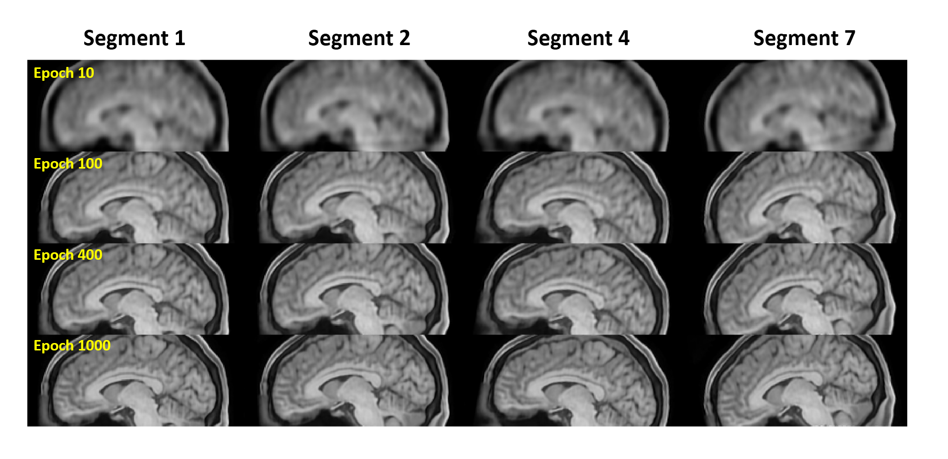
Intermediate training results during different epochs are shown in Figure 2. The proposed algorithm outperformed conventional TV-based algorithm for both 2D (Figure 3, NMSE: 0.0066 ± 0.0009 vs 0.034 ± 0.004, P < 0.01; PSNR: 29.60 ± 0.74 vs 22.06 ± 0.57, P < 0.01; SSIM: 0.89 ± 0.014 vs 0.71 ± 0.013, P < 0.01) and 3D imaging (Figure 4, NMSE: 0.0067 ± 0.0008 vs 0.037 ± 0.004, P < 0.01; PSNR: 32.40 ± 1.63 vs 25.70 ± 1.66, P < 0.01; SSIM: 0.89 ± 0.01 vs 0.65 ± 0.01, P < 0.01). Besides, the proposed algorithm has good tolerance to motion estimation errors when SNR decreased from 100 dB to 1 dB (Figure 5).

The CNN-based motion correction algorithm is more robust than conventional TV-based algorithm when more than 5% images were missing, and preserved good image quality with even 20% data missing (NMSE = 0.0087 for 2D imaging and NMSE = 0.0083 for 3D imaging).

Conclusion

Acknowledgements

References

1. Manduca A, McGee K, Welch E, Felmlee J, Grimm R, Ehman R. Auto-correction in MR Imaging: adaptive motion correction without navigator echoes. Radiology 2000;215: 904-909.


2. Atkinson D, Hill DL, Stoyle PN, Summers PE, Keevil SF. Automatic correction of motion artifacts in magnetic resonance images using an entropy focus criterion. IEEE Trans Med Imaging 1997;16: 903-910.

3. Atkinson D, Hill DL, Stoyle PN, Summers PE, Clare S, Bowtell R, Keevil SF. Automatic Compensation of Motion Artifacts in MRI. Magn Reson Med 1999;41: 163-170.

4. Lin W, Ladinsky G, Wehrli F, Song HK. Image metric-based correction (autofocusing) of motion artifacts in high-resolution trabecular bone imaging. J Magn Reson Imaging 2007;26: 191-197.

5. Haskell MW, Cauley SF, Wald LL. TArgeted Motion Estimation and Reduction (TAMER): Data Consistency Based Motion Mitigation for MRI Using a Reduced Model Joint Optimization. IEEE Trans Med Imaging. 2018;37: 1253-1265.

6. Loktyushin A, Nickisch H, Pohmann R, Schölkopf B. Blind retrospective motion correction of MR images. Magn Reson Med 2013;70: 1608-1618.

7. McGee KP, Manduca A, Felmlee JP, Riederer SJ, Ehman RL. Image metric-based correction (autocorrection) of motion effects: analysis of image metrics. J Magn Reson Imaging 2000;11: 174-181.

8. Cheng JY, Alley MT, Cunningham CH, Vasanawala SS, Pauly JM, Lustig M. Nonrigid motion correction in 3D using autofocusing with localized linear translations. Magn Reson Med. 2012;68: 1785-97.

9. The Human Connectome Project. Available at: https://www.humanconnectome.org/.

10. Van Essen DC, Smith SM, Barch DM, Behrens TE, Yacoub E, Ugurbil K; WU-Minn HCP Consortium. The WU-Minn Human Connectome Project: an overview. Neuroimage 2013;80: 62-79.

11. Ashburner J. A Fast Diffeomorphic Image Registration Algorithm. Neuroimage 2007;38:95-113.