4424
Three-dimensional motion correction in Magnetic Resonance Fingerprinting (MRF)1Italian National Institute of Nuclear Physics, Pisa, Italy, 2IMAGO7 research Foundation, Pisa, Italy, 3Department of Physics, University of Pisa, Pisa, Italy, 4Computer Science department, Technical University of Munich, Munich, Germany, 5GE Healthcare, Munich, Germany, 6IRCCS Stella Maris, Pisa, Italy
Synopsis
Two-dimensional MRF is considered to be less sensitive to in-plane motion than conventional imaging techniques. However, in scanning populations prone to rapid and extensive motion, challenges remain. Here, we suggest a two-step 3D MRF procedure that includes the correction of subject motion during the reconstruction. In the first step, we reconstruct the data in small segments consisting of images with equal contrast and calculate the between-segment motion. In the second step, we perform motion correction and use corrected images for matching with dictionary. This results in higher quality of reconstructed images and better precision of quantitative maps.
Introduction
MR Fingerprinting has been successfully used to quantify relaxation times of different tissues1. Although it was suggested that MRF is less sensitive to motion than conventional acquisition schemes1, excessive motion may result in the incorrect estimation of tissue parameters. The effect of motion has been recently investigated in 2D MRF and it was proved that accounting for subject movements improves the estimation of quantitative maps2. A different study also suggested that through-plane motion affects the estimation of T2 values, decreasing the validity of quantitative estimates3. To mitigate this problem, we developed a 3D MRF pipeline that accounts for three-dimensional motion.Methods
3D MRF sequence
Data was acquired on a clinical 1.5 T scanner (HDx, GE Healthcare). In our 3D-MRF acquisition we sampled random radial directions at each frame (Fig 1A.) with constant TE/TR. Each segment of the data was acquired with a pattern of flip angles (Fig. 1B). Replicating this design across the acquisition results in segments of equal contrasts with the same angular sampling density in the 3D k-space. Images from each segment, combined together, create a fully reconstructed image. We use a singular value decomposition to compress acquired frames in k-space to singular values4. The final images form a 128x128x128 volume of (1.5 mm)3 voxels.
Simulation
Data from a phantom were collected with a single-segment acquisition. Motion was simulated by shifting and rotating the trajectories before the reconstruction. A timecourse of 3D volumes, formed by the reconstructed volume with no motion, followed by the volumes with simulated motion, was generated. The 3D motion correction algorithm implemented in AFNI was applied5.
In vivo experiment
Two subjects participated to this study (case A and B), each acquired twice, with a 48-segment scheme. In the first acquisition, subjects were instructed to stay still, while in the second they randomly moved their heads. The processing pipeline on the data with deliberate motion was as follows. 1) Each acquisition was first reconstructed segment by segment to form a timeseries of 3D volumes. During reconstruction, the k-space was apodised by a 3D Gaussian (FWHM=16 k-space points) to decrease noise and facilitate motion correction. 2) Between-segment motion was estimated from the magnitude data and the transformation matrix was applied to the complex data of each segment. 3) MRF dictionary fitting was run on motion-corrected images and uncorrected images with motion artifacts. Results were compared with the dataset without voluntary motion.
Results
Fig. 2 proves that a motion correction algorithm can correctly estimate the simulated movements (Fig. 2A), and shows the effect of motion correction applied to phantom data (Fig. 2B).
Fig. 3 shows an improvement of the in vivo data reconstructed with the motion correction algorithm. Not only the anatomical landmarks are of higher quality but also T1 maps comprise of higher detail. In Fig. 4 we correlate quantitative estimates between the datasets, and in both cases after the correction values are closer to the ground truth. To obtain a spatial map of the fitting error, we plot the correlation values between dictionary and acquired data as a map for the case A (Fig. 5A). We observe that the correction increases the correlation values globally (Fig. 5), especially in areas highly affected by motion.
Discussion
Estimation of 3D-MRF parameters can be improved by applying motion correction while reconstructing the data, improving quantitative data both for T1 and T2. However, we observe that extreme motion (case B) affects more the T2 values, which may be the results of intra-segment misalignment as suggested before3. Our pipeline only accounts for movements between segments ignoring motion artifacts, that are present during the acquisition of a single segment. To account for intra-segment motion, one could discard the blurred segments that result in worse agreement with the baseline image. Another possibility might be to divide the data into smaller segments, to decrease the acquisition time of a segment. This however might result in lower SNR and failure of the motion algorithm to correctly estimate the movements. Our data comprises of a quick acquisition protocol for 3D MRF (less than 5 minutes). The same procedure could be applied to different k-space trajectories with properly ordered interleaves and longer acquisitions as our motion correction is insensitive to number of segments and trajectory used.Conclusions
We suggest a new type of 3D MRF and motion correction pipeline. After accounting for subject movement, the quality of the reconstructed images improves and estimation of quantitative values is closer to the non-motion condition.Acknowledgements
No acknowledgement found.References
- Ma, D., et al., Magnetic resonance fingerprinting.Nature, 2013. 495(7440): p. 187-92.2.
- Cruz, G., et al., Rigid motion-corrected magnetic resonance fingerprinting.Magn Reson Med, 2018.3.
- Yu, Z., et al., Exploring the sensitivity of magnetic resonance fingerprinting to motion.Magn Reson Imaging, 2018. 54: p. 241-248.4.
- McGivney, D.F., et al., SVD compression for magnetic resonance fingerprinting in the time domain.IEEE Trans Med Imaging, 2014. 33(12): p. 2311-22.5.
- Cox, R.W., AFNI: software for analysis and visualization of functional magnetic resonance neuroimages.Comput Biomed Res, 1996. 29(3): p. 162-73.
Figures

Fig 1A: Sequence diagram for 3D radial trajectories. Spokes were acquired with randomized angles (theta, phi).
Fig 1B: Flip angle pattern that presents the idea of equal contrast segments. Inversion pulse was present before each segment.
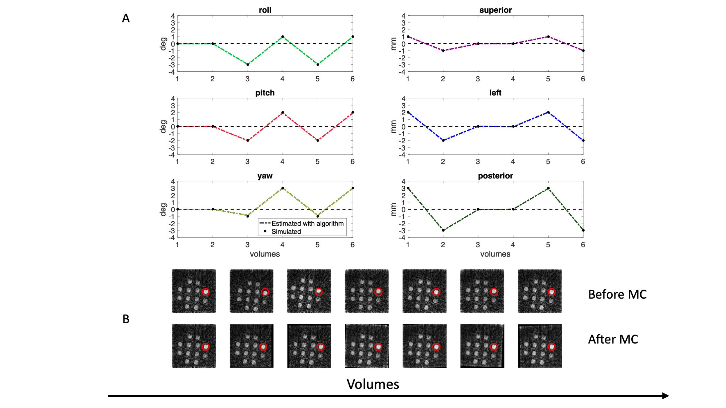
Fig. 2A: Presents the simulated and estimated motion parameters.
Fig. 2B: Illustrates the volumes before and after applying the motion correction (images of the 1st singular value). First image is the reference, next two volumes consist only of translation followed by two of rotation and last two of both translation and rotation. Red circles are used to appreciate the applied correction.


Fig. 5A: Correlation values from dictionary matching for the middle axial slice for the case A.
Fig. 5B: Histogram of the same parameter for the presented slice (red before correction, green after the correction). Straight lines indicate the mean.