4416
Towards in-vivo voxel-wise parcellation of human brain cortexShahrzad Moeiniyan Bagheri1, Viktor Vegh1, and David Reutens1
1Centre for Advanced Imaging, The University of Queensland, St Lucia, Australia
Synopsis
The research aims to establish the feasibility of developing an automated method for in vivo voxel-wise parcellation of the human brain cortex. We combined our previously proposed residual analysis Magnetic Resonance Fingerprinting (MRF) approach with supervised classification. We show that extraction of a feature vector from a patch of voxels about a voxel of interest improves prediction accuracy by about 10%, as measured using the Area Under the Curve (AUC) metric. Our approach leads to an increase in the prediction accuracy rate for areas of distinct microstructural heterogeneity, such as the primary motor cortex.
Introduction
The importance of developing accurate anatomical maps of the human brain has been highlighted in a multitude of studies. Such maps can have significant impact in, for example, neurosurgical decision making processes. 1, 2 Despite this critical need, a method has not been developed to date which works with MRI human brain in vivo data. Here, we further develop our previous work 3 on using Magnetic Resonance Fingerprinting (MRF) 4 for distinguishing microstructural variations between different cortical areas, with the goal of voxel-level classification of the human brain cortex.Methods
We acquired data from 7 healthy participants using a 7T whole-body MRI research scanner (Siemens Healthcare, Erlangen, Germany), as described previously. 3 We applied the following classification methods: K-Nearest Neighbours (KNN), Linear Support Vector Machine (L-SVM), Radial Basis Function kernel SVM (RBF-SVM) and Random Forests (RF). We opted to use classify the following cortical areas: BA2 (primary somatosensory cortex), BA4 (primary motor cortex) and BA6 (premotor cortex). We used the Area Under the Curve (AUC) metric to evaluate model performance instead of accuracy, since the latter can misrepresent when dealing with unbalanced training sets. 5 We have previously shown the autocorrelation values of the residual MRF signals to be able to differentiate the microstructural differences between three cortical areas: BA2, BA4 and BA6. 3 To calculate autocorrelations, we normalised both the acquired MRF signals and the residual MRF signals, resulting in normalised autocorrelations (between -1 and +1). Using this notion, we formed feature vectors for voxels of 1000 repetitions (1000 feature vector elements for each voxel, each element being the autocorrelation of the residual signal with a specific lag). The importance of selecting and extracting a proper feature set has been studied in a variety of machine learning applications. 6 To satisfy this need, we implemented two different approaches. Firstly, we simply extracted the features (i.e. autocorrelation of the residual signal) associated with a single voxel under consideration as a sample in the training set. Secondly, we investigated the additional use of a patch of surrounding voxels (3x3 region) and, a feature vector for a voxel was generated by sequential concatenation of the first 251 autocorrelations from the voxel neighbourhood and the voxel itself. Finally, we decided on a suitable metric to statistically characterise the residual MRF signals resulting from our already established pipeline. 3 Through a feature selection process, we subsequently reduced the number of features to the set that showed the highest contribution towards improving the classifier’s performance. We then performed model selection, as we also did for the single voxel approach, using 5-fold cross-validation method and by considering AUC as the evaluation score. We should note that class labels for all samples have been derived from the binary masks of the three cortical areas available in Juelich histological atlas of the human brain, 7 after transformation from the MNI space 8 to the native MRF space.Results and Discussion
Figure 1 provides the single-voxel feature selection and model selection results. RBF-SVM was found to perform best, with average AUC=0.76 (regularisation parameter C=118, kernel width parameter gamma=0.3). For all models the autocorrelations beyond 500 lags do not provide marked improvements in performance. The first 251 lags seem to have the highest influence, which is the number used in the patch-based analysis. The patch-based results are provided in Table 1, where the RBF-SVM model outperformed all other models investigated in this study (AUC=0.81; regularisation parameter C=28 and kernel width gamma=0.1). Confusion matrices for the RBF-SVM approach are provided in Figure 2 for single-voxel and patch-based feature selection. We found the TPR (True Positive Rate) of predictions to improve by using patch features (e.g. BA4 increase to 0.70 from 0.61). This finding is particularly important, as BA4 has higher micro-architectonic heterogeneity than the other two areas, which makes classification challenging. 9 Additionally, the FPR (False Positive Rate) for each area is consistent with the microstructural similarity and dissimilarity of these areas established using histological studies. 10, 11 For example for the case when the true class is BA4, the FPR for BA6 is much larger than for BA2, which suggests that BA4 is micro-architectonically more similar to BA6 than to BA2.Figure 3 depicts the distribution of the predicted class labels for an unseen set of samples from MRF images, using RBF-SVM based classification and voxel patches.Conclusion
We showed the feasibility of developing a machine learning classification approach based on residual MRF signals for the purpose of automatic parcellation of the human brain cortex in vivo. We found features based on a patch of voxels led to higher prediction accuracy in comparison to a single voxel approach.Acknowledgements
The authors acknowledge the facilities and scientific and technical assistance of the National Imaging Facility, a National Collaborative Research Infrastructure Strategy (NCRIS) capability, at the Centre for Advanced Imaging, The University of Queensland. VV and DR acknowledge support from the Australian National Health and Medical Research Council (NHMRC APP1104933) and from the Australian Research Council (DP140103593).References
- Duffau H. Lessons from brain mapping in surgery for low-grade glioma: insights into associations between tumour and brain plasticity. The Lancet Neurology. 2005;4(8):476-486.
- Magara A, Buhler R, Moser D, Kowalski M, Pourtehrani P, Jeanmonod D. First experience with MR-guided focused ultrasound in the treatment of Parkinson's disease. Journal of therapeutic ultrasound. 2014;2(1):11.
- Moeiniyan Bagheri S, Vegh V, Reutens D. Magnetic Resonance Fingerprinting (MRF) can reveal microstructural variations in the brain gray matter. Paper presented at: ISMRM, 2018; Paris.
- Ma D, Gulani V, Seiberlich N, et al. Magnetic resonance fingerprinting. Nature. 2013;495(7440):187.
- Chawla N, Japkowicz N, Kotcz A. Special issue on learning from imbalanced data sets. ACM Sigkdd Explorations Newsletter. 2004;6(1):1-6.
- Guyon I, Elisseeff A. An introduction to variable and feature selection. Journal of machine learning research. 2003;3(Mar):1157-1182.
- Eickhoff S. Jülich histological (cyto- and myelo-architectonic) atlas references. FSL. August 2012. Available at: HYPERLINK "http://fsl.fmrib.ox.ac.uk/fsl/fslwiki/Atlases/Juelich" http://fsl.fmrib.ox.ac.uk/fsl/fslwiki/Atlases/Juelich . Accessed 2016.
- Mazziotta J, Toga A, Evans A, et al. A four-dimensional probabilistic atlas of the human brain. Journal of the American Medical Informatics Association. 2001;8(5):401-430.
- Geyer GS, Ledberg A, Schleicher A, et al. Two different areas within the primary motor cortex of man. Nature. 1996;382(6594):805.
- Cohen-Adad J, Polimeni JR, Helmer KG, et al. T2* mapping and B0 orientation-dependence at 7 T reveal cyto-and myeloarchitecture organization of the human cortex. Neuroimage. 2012;60(2):1006-1014.
- Guillery R. Brodmann's ‘Localisation in the Cerebral Cortex. Journal of Anatomy. 2000;196(3):493-496.
Figures
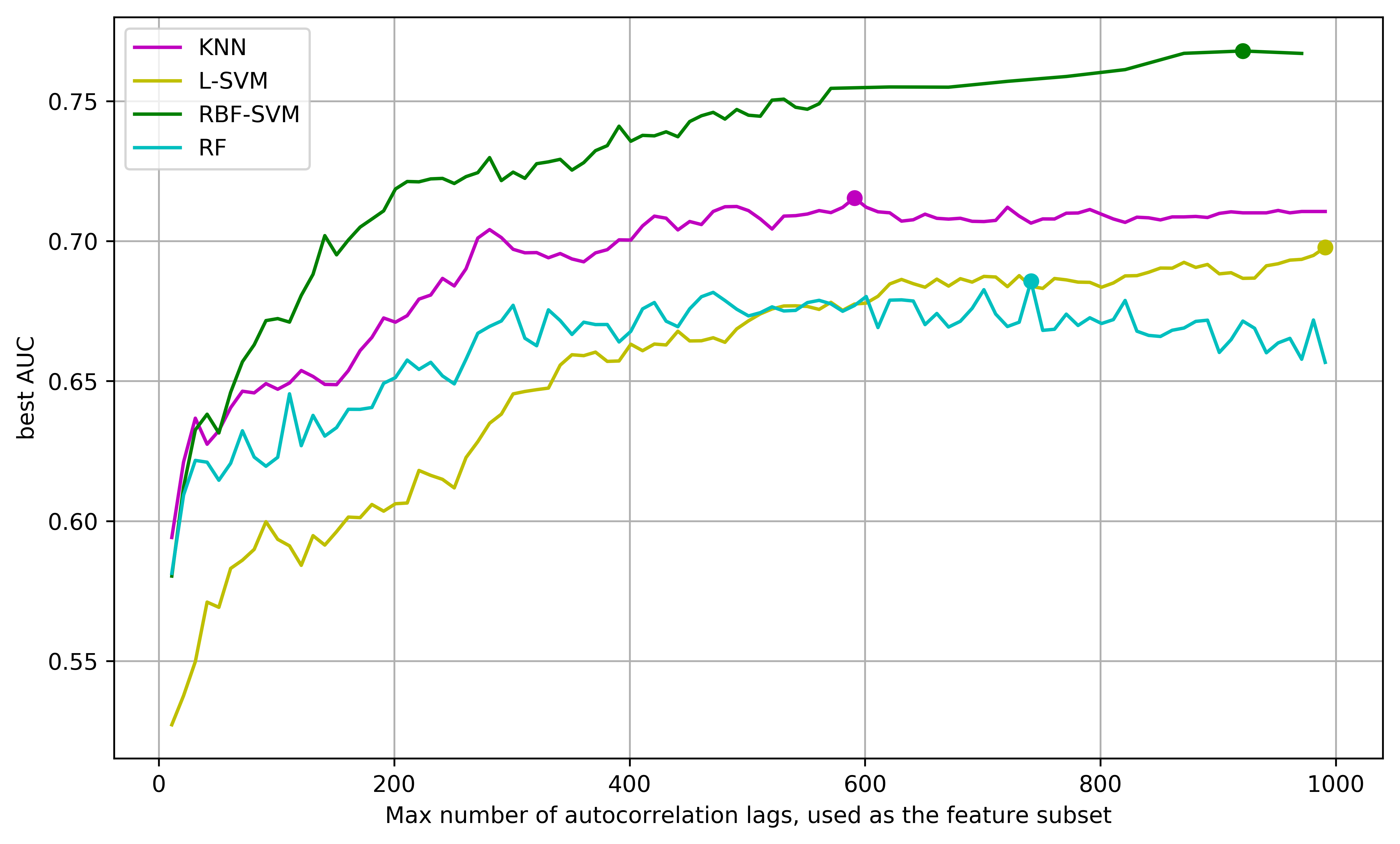
Figure 1. The best AUC scores of four supervised classification algorithms are compared when trained with different subset of autocorrelation values as feature vectors using the four classification methods: KNN, L-SVM, RBF-SVM and RF. The solid circle on each plot represents the subset of autocorrelations at which that model showed its best performance.
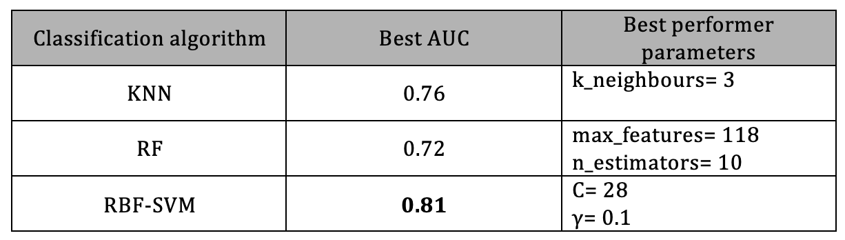
Table 1. The AUC of the three supervised classification methods using the patch approach.
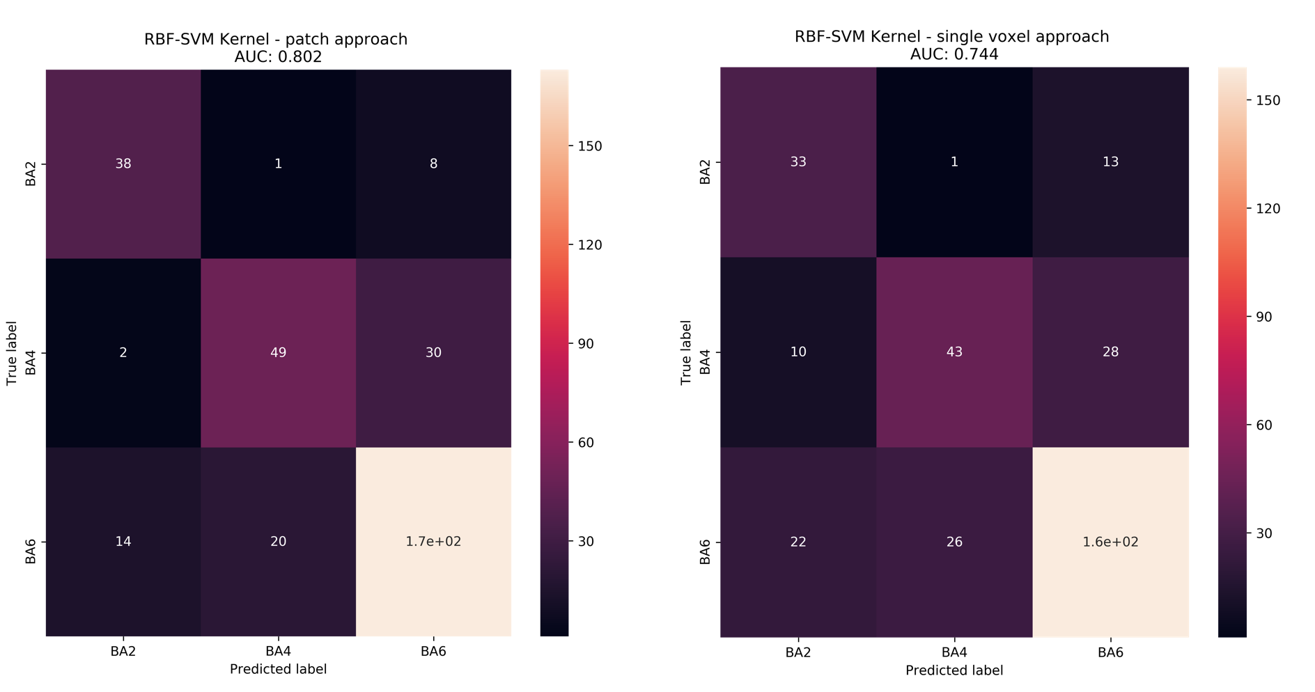
Figure 2. Confusion matrices for RBF-SVM with patch features (on the left) and the single voxel features (on the right). The AUC score of each classifier is stated at the top. Cell values represent the number of samples within the test set that have been classified as the class identified at the bottom of each column.
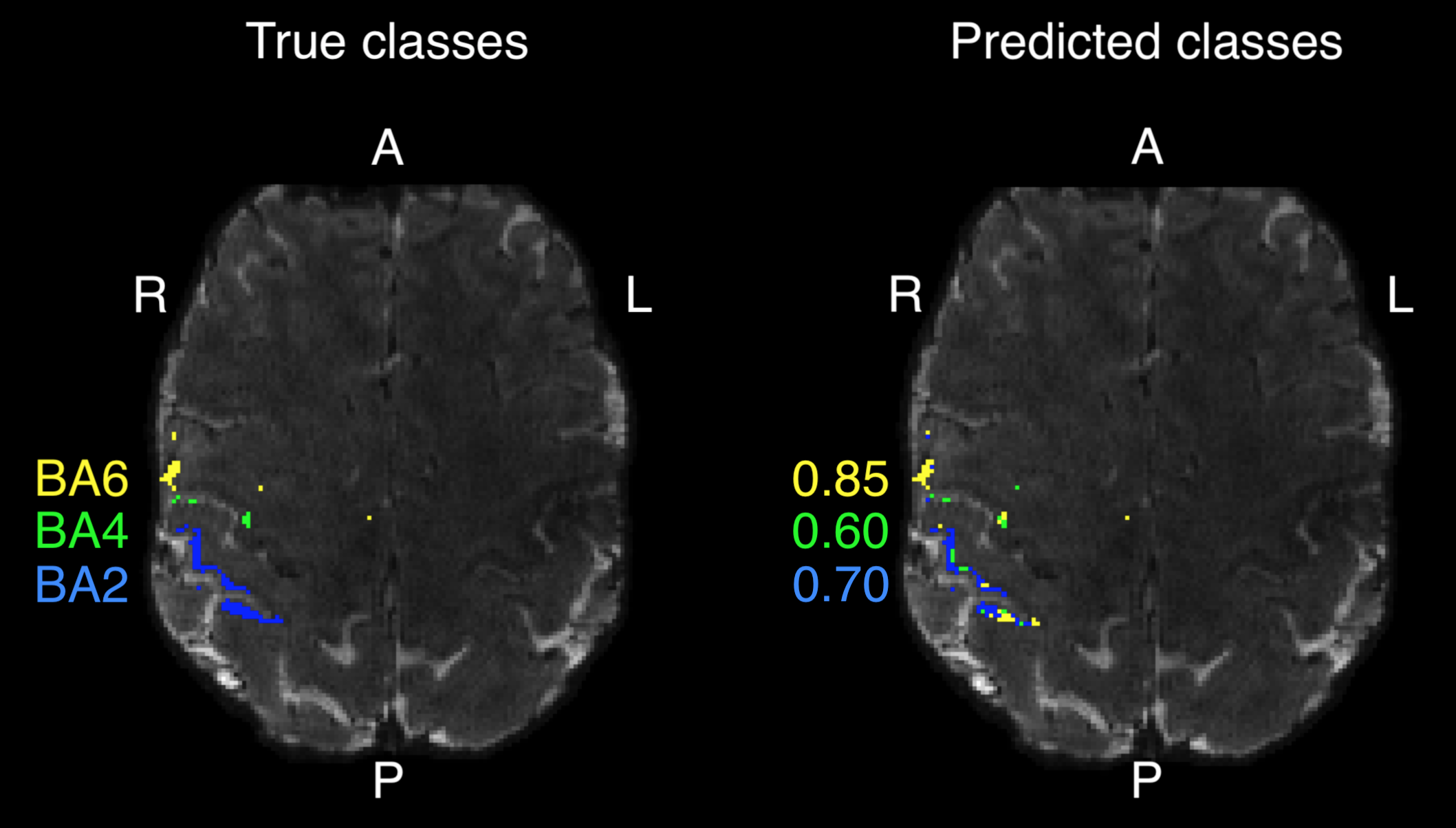
Figure 3. Using RBF-SVM and the patch approach, the voxels from one slice of a MRF scan (this participant was excluded from the training) are classified into BA2 (blue), BA4 (green) and BA6 (yellow). The TPR of predictions for each class are represented by the same colours as their class labels. On the left, the true classes extracted from the Juelich histological brain atlas have been provided for reference.