4401
A fast, joint sparsity constraint algorithm for improved myelin water fraction mapping1TU Berlin, Berlin, Germany, 2Philips, Hamburg, Germany, 3Philips Research Europe, Hamburg, Germany
Synopsis
A new method for myelin water fraction mapping from multi-echo spin echo data using a joint sparsity constraint is proposed, which is faster than previously proposed methods. This method is based on the assumption that the T2 spectrum is sparse and consists of a common small set of discrete relaxation times for all voxels. The method finds an estimation of the flip angle inhomogeneity map from the data itself, to remove the bias caused by B1 inhomogeneities. The proposed method is compared to state of the art MWF approaches in 3T brain measurements.
Introduction
Myelin water fraction (MWF) mapping provides the means to assess myelin changes in cerebral white matter in vivo. One approach to MWF mapping is multi-component T2 analysis from multi-echo spin-echo (MESE) data, in which the T2 values below a certain threshold are assumed to belong to myelin water. The original method [1] based on the non-negative least squares(NNLS) algorithm [2] assumes non-negativity of the solution and proposes a smooth distribution to improve the noise-robustness. Later, spatial regularisation of the distribution was proposed to further improve the robustness [3].
The MESE measurement is sensitive to flip angle inhomogeneities (FAI) due to B1-variations. Methods including FAI compensation [4,5] lead to improved results, but have rather long computation times.
In this work, we propose a new, faster method for calculating the MWF including FAI-compensation using joint sparsity.
Methods
The main premise of the proposed method is that the measured MESE signals can be represented as a linear combination of a few basis signals, corresponding to different components (e.g. myelin water, intra and extra-cellular water, free water), and that these components are the same for all voxels in the scan.
Assuming there are no flip angle inhomogeneities, the proposed method can be formulated as the following minimization problem:$$\min_{\mathbf{C}\in\mathbb{R}_{\geq 0}^{N\times J}}\lVert\mathbf{X}-\mathbf{D}\mathbf{C}\rVert^2_F+\lambda\sum_{i=1}^N\lVert \mathbf{c}^i\rVert_0$$Here $$$\mathbf{X}$$$ is a matrix containing the measured MESE signals for $$$J$$$ voxels, $$$\mathbf{D}$$$ is a matrix containing the simulated temporal signal evolutions for $$$N$$$ different T2 values, each column of $$$\mathbf{C}$$$ contains the coefficients of the $$$N$$$ components for a voxel and $$$\mathbf{c}^i$$$ denotes the ith row of $$$\mathbf{C}$$$. The parameter $$$\lambda$$$ balances the approximation error and the number of components. The joint sparsity problem without non-negativity constraints has been studied extensively in distributed compressed sensing literature [6]–[10].
To solve this problem we propose a new
algorithm, the Sparsity Promoting Iterative
Joint NNLS (SPIJN) algorithm. Since it is not computationally feasible to directly solve for the $$$\ell_0$$$-norm regularized
problem, we use an iteratively reweighted scheme that approximates this
regularization. The reweighting puts higher weight to components which are jointly
used making them more likely to be selected in the next iteration. We use the
weights $$$w_i=\lVert\mathbf{c}^i\rVert_2+\epsilon$$$ (here $$$\epsilon=10^{-4}$$$)
($$$i=1,…,N$$$), which is the $$$\ell_2$$$-norm of the coefficients over the FOV. The core of each iteration is formed by the NNLS
algorithm [2], which is used to
solve the reweighted NNLS problem $$$\min_{\mathbf{C}\in\mathbb{R}_{\geq 0}^{N\times~J}}\lVert\tilde{\mathbf{X}}-\tilde{\mathbf{D}}\mathbf{C}\rVert^2_F$$$. The following
steps are performed in each iteration of the algorithm:$$\mathbf{W}_{k+1}=\operatorname{diag}(\left(\mathbf{w}\right)_{k+1}^{1/2}),\\\tilde{\mathbf{D}}_{k+1}=\begin{bmatrix}\mathbf{D}\mathbf{W}_{k+1}\\\lambda\mathbf{1}^T\end{bmatrix},\\\tilde{\mathbf{X}}=\begin{bmatrix}\mathbf{X}_{k+1}\\\mathbf{0}^T\end{bmatrix},\\\tilde{\mathbf{C}}_{k+1}=\operatorname{argmin}_{\mathbf{C}\in\mathbb{R}_{\geq0}^{N\times~J}}\lVert\tilde{\mathbf{X}}-\tilde{\mathbf{D}}\mathbf{C}\rVert^2_F,\\\mathbf{C}_{k+1}=\mathbf{W}_{k+1}\tilde{\mathbf{C}}_{k+1}.$$To account for FAI, first a large set of
signal evolutions corresponding
to each combination of T2 and FAI (also called a dictionary) is computed
using the extended phase graph algorithm [11]. The FAI values for each voxel are
determined by finding the best match between the measured signal and the
dictionary of simulated signals, similar to [12]. Then, for each voxel, the matrix $$$D$$$
is selected as the submatrix containing the estimated FAI and all T2 values,
and the SPIJN algorithm is performed with the selected submatrices, effectively
compensating for the FA inhomogeneity. The
dictionary in this work included T2 values ranging from 10ms to 5s
logarithmically spaced with 140 steps and FAI of 0.6 to 1 in 100 steps.
The proposed method was evaluated in a MESE brain dataset. The dataset was acquired on a 3T MR-scanner (Ingenia 3.0T, Philips, Best, The Netherlands) with the following parameters: 48 echoes, ΔTE=8ms,TR=1200ms,FOV=240x205x72mm3,resolution=1.25x1.25x8mm3 and 9 slices.
For comparison, MWF-maps were also estimated with two other approaches, the standard NNLS algorithm [2] with the FAI-map estimated from our approach and the B1-compensated regularized-NNLS (regNNLS) method [5].
Results and discussion
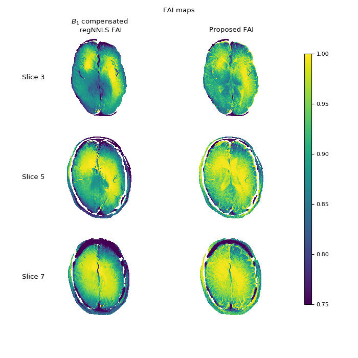
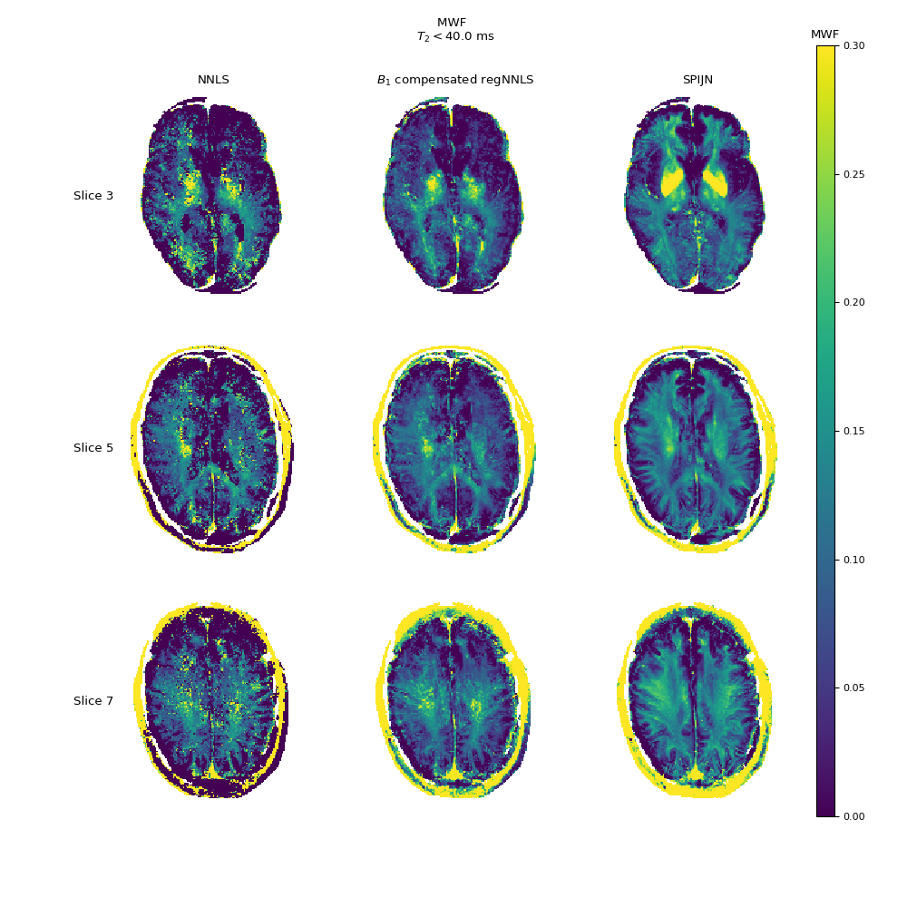
Figs1,2 show the results for the 3T data for three slices. NNLS took 21 seconds per slice, regNNLS 22 minutes, and SPIJN 45 seconds on a simple laptop (IntelCore i5-6300U CPU @2.40GHz 2 cores, 4 threads).
The FAI-maps of both methods are similar, however, our FAI-maps show a little bit of brain structure, which is a drawback of this relatively simple approach assuming a single T2/FAI component for each voxel. In the ventricles such B1 offset has been observed before [13]. To prevent this, spatial smoothing could be applied to the FAI-map.
The NNLS MWF-maps show noise amplification, which is reduced by the regNNLS method, with the drawback of longer computation times. The SPIJN MWF-maps show better left-right-symmetry than the regNNLS maps.
Conclusion
The proposed FAI-map approximation combined with the SPIJN algorithm using joint sparsity constraints gives results comparable to previously proposed methods with the advantage of practically feasible computation times.Acknowledgements
No acknowledgement found.References
[1] K. P. Whittall and A. L. MacKay, “Quantitative interpretation of NMR relaxation data,” J. Magn. Reson. 1969, vol. 84, no. 1, pp. 134–152, Aug. 1989.
[2] C. L. Lawson and R. J. Hanson, Solving least squares problems. SIAM, 1974.
[3] D. Hwang and Y. P. Du, “Improved myelin water quantification using spatially regularized non-negative least squares algorithm,” J. Magn. Reson. Imaging, vol. 30, no. 1, pp. 203–208, Jun. 2009. [4] D. Kumar, S. Siemonsen, C. Heesen, J. Fiehler, and J. Sedlacik, “Noise robust spatially regularized myelin water fraction mapping with the intrinsic B1-error correction based on the linearized version of the extended phase graph model,” J. Magn. Reson. Imaging, vol. 43, no. 4, pp. 800–817, Apr. 2016.
[5] T. Prasloski, B. Mädler, Q.-S. Xiang, A. MacKay, and C. Jones, “Applications of stimulated echo correction to multicomponent T2 analysis,” Magn. Reson. Med., vol. 67, no. 6, pp. 1803–1814, Jun. 2012.
[6] M. F. Duarte, S. Sarvotham, D. Baron, M. B. Wakin, and R. G. Baraniuk, “Distributed Compressed Sensing of Jointly Sparse Signals,” 2005, pp. 1537–1541.
[7] S. F. Cotter, B. D. Rao, Kjersti Engan, and K. Kreutz-Delgado, “Sparse solutions to linear inverse problems with multiple measurement vectors,” IEEE Trans. Signal Process., vol. 53, no. 7, pp. 2477–2488, Jul. 2005.
[8] J. A. Tropp, A. C. Gilbert, and M. J. Strauss, “Algorithms for simultaneous sparse approximation. Part I: Greedy pursuit,” Signal Process., vol. 86, no. 3, pp. 572–588, Mar. 2006.
[9] J. A. Tropp, “Algorithms for simultaneous sparse approximation. Part II: Convex relaxation,” Signal Process., vol. 86, no. 3, pp. 589–602, Mar. 2006.
[10] J. D. Blanchard, M. Cermak, D. Hanle, and Y. Jing, “Greedy Algorithms for Joint Sparse Recovery,” IEEE Trans. Signal Process., vol. 62, no. 7, pp. 1694–1704, Apr. 2014.
[11] J. Hennig, “Multiecho imaging sequences with low refocusing flip angles,” J. Magn. Reson. 1969, vol. 78, no. 3, pp. 397–407, Jul. 1988.
[12] N. Ben‐Eliezer, D. K. Sodickson, and K. T. Block, “Rapid and accurate T2 mapping from multi–spin-echo data using Bloch-simulation-based reconstruction,” Magn. Reson. Med., vol. 73, no. 2, pp. 809–817, Feb. 2015.
[13] W. M. Brink, P. Börnert, K. Nehrke, and A. G. Webb, “Ventricular B1+ perturbation at 7 T – real effect or measurement artifact?,” NMR Biomed., vol. 27, no. 6, pp. 617–620, Jun. 2014.
Figures