4383
Quantifying liver function using artificial neural networks to estimate gadoxetic-acid uptake rate in temporally sparse gadoxetic-acid enhanced MRI1Biomedical Engineering, University of Michigan, Ann Arbor, MI, United States, 2Radiation Oncology, University of Michigan, Ann Arbor, MI, United States
Synopsis
Though methods exist for quantifying regional liver function from dynamic gadoxetic-acid enhanced (DGE) MRI, errors are introduced when using the clinically typical temporally sparse acquisition scheme (6 volumes over 20 minutes) relative to a temporally dense dynamic acquisition (volumes every 5-10 sec over a similar period). This motivates a data driven approach. An artificial neural network (ANN) was trained to reproduce the results of the fully characterized analysis using only the restricted dataset. Across the patients evaluated the ANN solution resulted in lower mean and median WMAPE, as well as a reduction in MSE in most cases.
Introduction
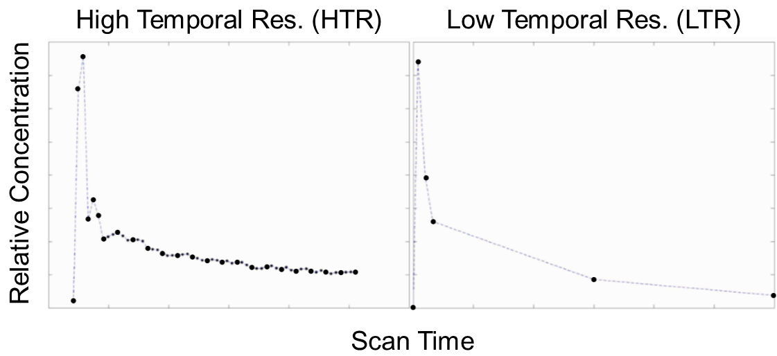
A previous study develops a single input two compartment model (LSITCM) to robustly estimate Gadoxetic acid uptake rate (k1) from DGE MRI in the liver (Simeth et al.). The LSITCM can be applied to clinical data having as few as 6 acquired image volumes. However, early volumes may be obtained before the assumptions of the LSITCM are true, confounding the estimate. This study aims to train an artificial neural network (ANN) for prediction of k1 using sparsely sampled 6 low-temporal resolution (LTR) image volumes with varying time points (see figure 1).Methods
Thirty-two high-temporal resolution (HTR) (figure 1) DGE MRI scans of the liver were acquired up to 20 min in 25 patients with hepatic cancers on a 3T scanner. To estimate k1, the HTR DGE signals were fitted to the LSITCM:
$$\overbrace{\frac{(1-Hct)C_{t}(t)}{C_{a}(t)}}^{\textrm{y}} \approx \overbrace{v_{dis} k_1}^{\textrm{slope}} \overbrace{\frac{\int_0^t C_{a}(\tau) d\tau }{C_{a}(t)}}^{\textrm{x}} + \overbrace{v_{dis}}^{\textrm{intercept}} [1]$$
where Ct and Ca are contrast concentrations of artery and tissue, respectively, vdis is a distribution volume, and Hct is hematocrit. To train an ANN, a population of voxels was randomly selected using100,000 voxels from each liver of 32 exams. To create the LTR DGE data, a time sampling scheme was used to select 6 time points. The initial 4 points started at zero and were uniformly spaced 5 to 50 seconds apart. Each of the initial 4 points was further perturbed by a fraction of their spacing. An intermediate point and terminating point were randomly selected from the central 50% and final 10% of the acquisition duration. The time variations of the time points prevents an identical x vector across all voxels in each exam. Intensities of the input curves at the 6 selected time points were defined through mean values over a 14 second period centered on the selected times using a linear interpolation. Then, x and y vectors were created using equation [1]. A small amount of noise was added to the x and y vectors for each voxel, to prevent overfitting. After removing the zero initial points, the x and y vectors were combined to form the input to the ANN. In addition to input and output layers, the ANN had 4 hidden layers, 2 with 10 neurons, followed by 2 with 5 neurons. The feed forward NN was trained with targets of k1 values from fitting the HTR dataset to equation [1]. The network was trained in Matlab using Levenberg-Marquardt backpropagation. A leave-one-out cross-validation was performed to evaluate k1 values of each patient’s exams using the ANN trained by only the other patient’s data. During ANN training, 75% of 2 million voxels of data were used for training and 25% for validation. Finally, to compare with the k1 values estimated from the ANN, the input LTR curves were directly fitted to the LSITCM. To test the model, both LSITCM and ANN solutions were applied to with the time interval of early points varied from 15 s to 35 s, maintaining the final point at the end of the acquisition, and choosing the intermediate point exactly equidistant.
Results
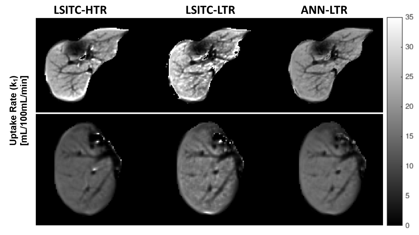
The leave-one-out cross validation showed that k1 values of 32 exams estimated by the ANN had a lower median and mean relative MSE (from -80.6% to -14.2%) than those from direct fitting of equation [1] (see figure 2). WMAPEs were also lower for the ANN as compared to direct fitting. Qualitatively, the ANN solutions reduced runaway noise and edge effects (see figure 3).
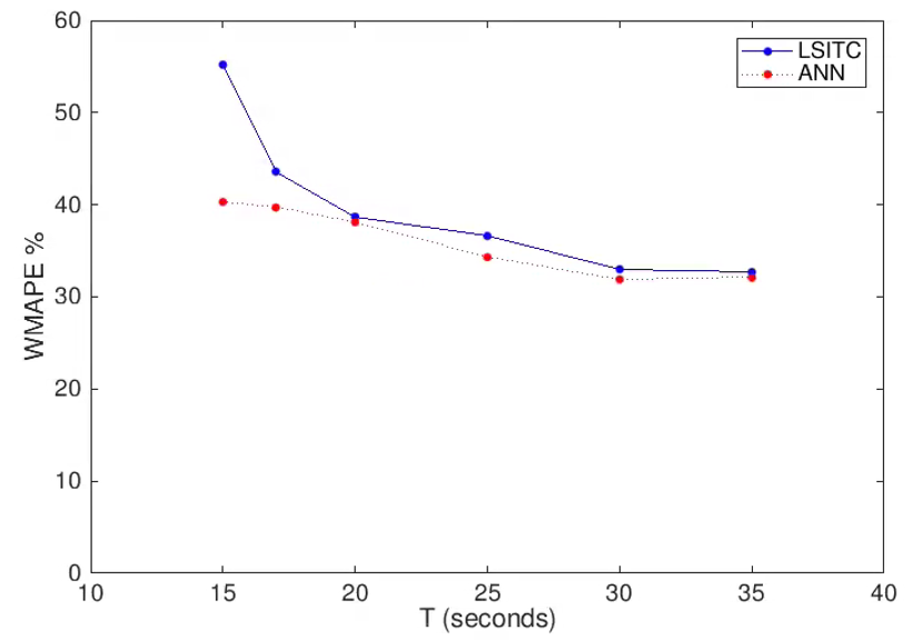
Both relative MSE and WMAPE of k1 by both methods decreased with an increase in the intervals between the first four time points, particularly the time of the 4th point. As seen in figure 4, the ANN approach was less sensitive to closely spaced early time points, but as the spacing increased both methods became comparable (mean WMAPE differed by only 0.64%).
Conclusion and Discussion
Data driven approaches to quantification of liver function provide tools for counteracting subtle biases and uncertainties in clinical data, that impact the solution in a complex manner. This study helps to quantify the error incurred in assessing LTR data, while demonstrating the viability of a data driven ANN approach. The artificial neural network substantially outperformed the LSITC model when the early post contrast points were tightly spaced. As the early points were spread out, both methods improved and the differences were reduced. This indicates that, if the uptake rate is desired, the early points should either be sufficiently spaced or augmented with successive points to ensure that early post contrast information is not entirely overwhelmed by transient perfusion effects.Acknowledgements
Supported by NIH grants R01 CA132834 and p01 CA059827.References
Simeth J, Johansson A, Owen D, et al. Quantification of liver function by linearization of a two‐compartment model of gadoxetic acid uptake using dynamic contrast‐enhanced magnetic resonance imaging. NMR in Biomedicine. 2018;31:e3913. https://doi.org/10.1002/nbm.3913Figures