4382
Phase Correction for Abdominal Quantitative Susceptibility Mapping with Bipolar Readout Gradients Sequence1Shanghai Key Laboratory of Magnetic Resonance, Shanghai, China, 2MR Collaboration NE Asia, Siemens Healthcare, Shanghai, China, Shanghai, China, 3Department of Radiology, Weill Medical College of Cornell University, New York, New York, USA, New York, NY, United States
Synopsis
Bipolar acquisition in abdominal multi-echo quantitative susceptibility mapping (QSM) could reduce echo-spacing and total scan time. However, the bipolar acquisition introduces phase error between odd and even echoes. A phase correction method in image domain was proposed to address this problem. We demonstrated the feasibility of generating a quantitative susceptibility map in human abdomen using bipolar multi-echo GRE sequence. Quantification analysis showed an excellent agreement between bipolar and unipolar methods.
Introduction
Bipolar acquisition in abdominal QSM could reduce echo-spacing and total scan time1,2. However, the bipolar readout gradients impose a phase between odd and even echoes which confounds water-fat separation and field map estimation. The principal phase error varies linearly along read and slice direction in image domain3. We proposed a method to correct this error, and then validated the feasibility as well as accuracy in human abdominal QSM.Methods
THEORY
For the bipolar multi-echo gradient echo sequence, the nth echo signal in terms of water, W, and fat, F with consideration of local field , signal decay and odd-even phase error is modeled as4:$$S(t_{n})=(W+F\sum_m^Mα_me^{i2π∆f_m t_n})e^{i2πf_B t_n}e^{-R_2^* t_n}e^{(-1)^n iθ}$$
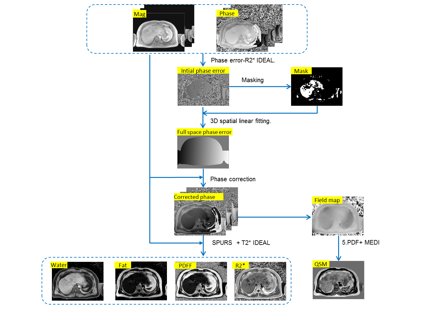
where water is assumed to be on resonance and the fat is modeled by M resonances with relative amplitudes and chemical shifts . The phase error as an additional unknown could be jointly estimated together with , using a iterative method similar to IDEAL 1, 5, 6. But the estimated error map is corrupted by plenty of noise-like points where estimations may be failed due to improper initial guess and too many unknowns, so only the reliable pixels were used for linear fitting along three directions to generate a full FOV phase error map. The fitted phase error map was then used to correct the original phase images. The processing procedure is illustrated in Figure 1.
Subjects and Acquisition
Six volunteers were recruited in this study with IRB approval from the institution and written informed consent from each subject. All imaging experiments were performed on a 3T MRI system (Prisma Fit, Siemens Healthcare) equipped with 18 channel torso coil. 3D axial multi-echo GRE data were acquired using a unipolar sequence (as the reference standard) and a bipolar sequence with the following imaging parameters for both sequences: TR = 11.3ms, TE1 = 1.07ms,ΔTE=1.79ms, pixel size = 1.8*1.8*3.5$$$mm^{3}$$$, matrix size = 224*196*52, FOV = 400*350$$$mm^{2}$$$, number of echoes=6, bandwidth =1060Hz/px. Each scan lasted 18 seconds and was readily completed during a single breath-hold at the end of exhalation.
Reconstruction
First, the odd-even phase errors in bipolar data were removed using the method mentioned above. Then, water-fat separation technique T2*-IDEAL7 with 6-peak fat model was performed to estimate the local field map both in unipolar and phase corrected bipolar data. The initial guess was achieved using SPURS8 that was specially designed for abdominal QSM. Finally, the background field was removed using projection onto dipole fields and the remaining magnetic field was processed to generate a susceptibility map using the morphology enabled dipole inversion algorithm (MEDI)9,10,11 .
Data analysis
Susceptibility, R2* and PDFF were measured using region of interest (ROI) analysis. Four ROIs for each subject were manually drawn on liver, subcutaneous fat, latissimus dorsi muscle and spleen in unipolar axial QSM slices using ITK-SNAP. The ROIs were away from major vessels, artifacts as well as tissue-tissue boundaries. Linear regression analysis and Bland Altman analysis were performed to compare unipolar and bipolar methods.
Results
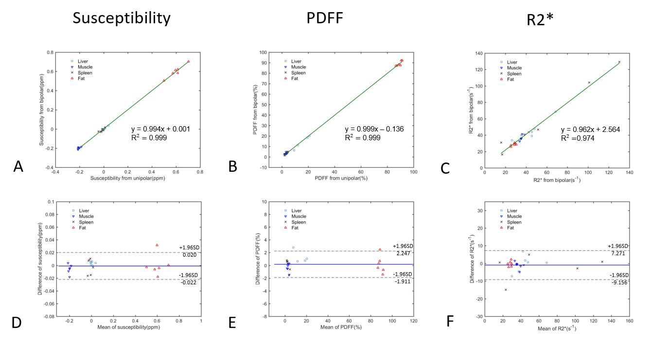
Figure 2A-C shows a clear linear correlation between bipolar and unipolar methods. Bland Altman plots the 95 % confidence interval of the mean measurement error between two methods with susceptibility value ranged from −0.022 to 0.020 ppm over the range of approximately -0.216 to 0.703 (Fig. 2D), PDFF ranged from -1.9% to 2.2% over the range of approximately 1.3% to 92.0% (Fig. 2E) , and R2* ranged from −9.2 to 7.3$$$s^{-1}$$$ over the range of approximately 16.3 to 129.4$$$s^{-1}$$$(Fig. 2F), respectively. There are no significant bias or trend between bipolar and unipolar methods. Both linear regression analysis and Bland Altman analysis suggest there's an excellent agreement between unipolar and bipolar methods.Discussion and Conclusion
The bipolar and unipolar methods used the same echo-spacing in this study. In fact, echo-sapcing could be further minimized in bipolar method. The misregistrations induced by the field inhomogeneity and chemical shifts were ignored for the following reasons. The measured local field inhomogeneity of 95% pixels range below 200Hz and chemical shift of lipid tissue at 3T is approximately 420Hz.Compared to 1kHz/px of receiver bandwidth, field inhomogeneity induced and chemical shifts induced misregistration were no more than 0.2 pixel and 0.5 pixel, respectively, which has a limited impact on reconstruction. In conclusion, we investigated the feasibility of generating a quantitative susceptibility map in human abdomen imaging from bipolar readout gradients sequence. Quantification analysis shows an excellent agreement between bipolar and unipolar methods.Acknowledgements
No acknowledgement found.References
[1]. Peterson, P. and S. Månsson, Fat quantification using multiecho sequences with bipolar gradients: Investigation of accuracy and noise performance. Magnetic Resonance in Medicine, 2014. 71(1): p. 219-229.
[2]. Sharma, S.D., et al., Quantitative susceptibility mapping in the abdomen as an imaging biomarker of hepatic iron overload. Magnetic Resonance in Medicine, 2015. 74(3): p. 673-683.
[3]. Li, J., et al., Phase-corrected bipolar gradients in multi-echo gradient-echo sequences for quantitative susceptibility mapping. Magnetic Resonance Materials in Physics, Biology and Medicine, 2015. 28(4): p. 347-355.
[4]. Peterson, P. and S. Månsson, Fat quantification using multiecho sequences with bipolar gradients: Investigation of accuracy and noise performance. Magnetic Resonance in Medicine, 2014. 71(1): p. 219-229.
[5]. Hernando, D., et al., Joint estimation of water/fat images and field inhomogeneity map. Magnetic Resonance in Medicine, 2008. 59(3): p. 571-580.
[6]. Reeder, S.B., et al., Iterative decomposition of water and fat with echo asymmetry and least-squares estimation (IDEAL): Application with fast spin-echo imaging. Magnetic Resonance in Medicine, 2005. 54(3): p. 636-644.
[7]. Yu, H., et al., Multiecho water-fat separation and simultaneous R2* estimation with multifrequency fat spectrum modeling. Magnetic Resonance in Medicine, 2008. 60(5): p. 1122-1134.
[8]. J., D., et al., Simultaneous Phase Unwrapping and Removal of Chemical Shift (SPURS) Using Graph Cuts: Application in Quantitative Susceptibility Mapping. IEEE Transactions on Medical Imaging, 2015. 34(2): p. 531-540.
[9]. Liu, T., et al., A novel background field removal method for MRI using projection onto dipole fields (PDF). NMR in Biomedicine, 2011. 24(9): p. 1129-1136.
10]. Liu, T., et al., Nonlinear formulation of the magnetic field to source relationship for robust quantitative susceptibility mapping. Magnetic Resonance in Medicine, 2013. 69(2): p. 467-476.
[11]. Liu, J., et al., Morphology enabled dipole inversion for quantitative susceptibility mapping using structural consistency between the magnitude image and the susceptibility map. NeuroImage, 2012. 59(3): p. 2560-2568.
Figures