Synopsis

Spiral and EPI are the most commonly used trajectories for imaging hyperpolarized ¹³C substrates. In this work, the two acquisition methods are compared with regard to B₀ and T₂^* effects for typical parameter sets used for in vivo imaging of the heart. While Spirals exhibit higher SNR, EPI trajectories show higher effective resolution with standard gradient system performance. The relative differences in SNR and resolution between the two trajectories reduce with the availability of high-performance gradients.

Introduction

Current single-shot acquisition schemes for magnetic resonance imaging of hyperpolarized ¹³C substrates in the heart are either based on Echo Planar Imaging (EPI)^1,2 or Spiral^3,4 k-space trajectories. In previous work, characterizations of EPI and Spiral trajectories have already been carried out regarding artifact behavior and different imaging resolutions.⁵ However, advantages and drawbacks of both trajectories in the presence of in vivo B₀ inhomogeneities as well as the detectability of local lesions in the heart as a function of acquisition scheme and experimental parameters have not been assessed so far. Accordingly, it is the objective of the present work to investigate effects of realistic in vivo B₀ inhomogeneities and T₂^* decay on EPI versus Spiral trajectories for detecting local lesions in the heart using hyperpolarized 13C imaging.

Methods

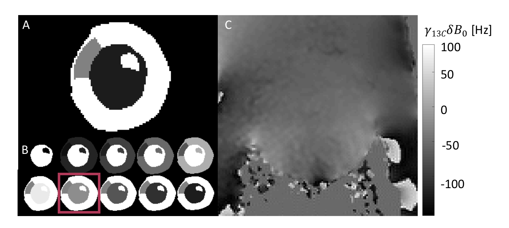
The extended cardiac-torso (XCAT)⁶ phantom of the left ventricle was augmented with an anteroseptal lesion as shown in Fig.-1A. The myocardial signal was derived from a simple perfusion model assuming an input function of substrate into the left ventricle followed by uptake into the myocardium as illustrated in Fig.-1B. The relative signal of the lesion was set to half the signal of remote myocardium. Acquisition of the resulting heart models was simulated using the following signal equation:

$$d(t)=\sum_{\vec{x}}{\rho(\vec{x})}e^{i\vec{k}(t)\vec{x}}e^{i\gamma\delta{B_0}(\vec{x})t}e^{-{t\over{T}_2^*(\vec{x})}}+\eta$$

with the resulting signals $$$d(t)$$$ stacked into vector $$$\vec{d}$$$, object $$$\rho(\vec{x})$$$, gyromagnetic ratio $$$\gamma$$$, sampling time $$$t$$$, relaxation time $$$T{_2}{^*}$$$, noise $$$\eta$$$, and B₀ variations $$$\delta{B}_0$$$ as shown in Fig.-1C. The resulting image $$$\vec{i}$$$ was obtained according to:

$$\vec{i}=F^HG\vec{d}$$

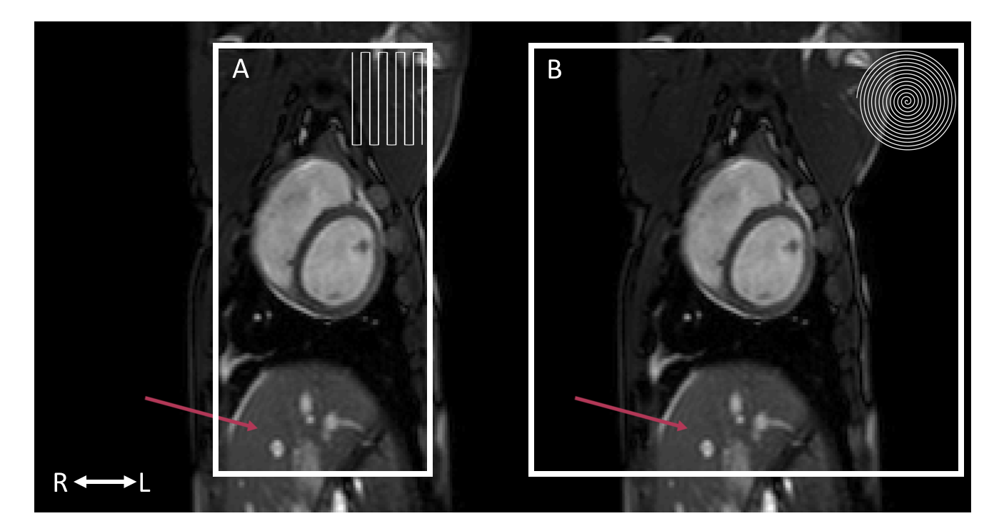
with Fourier operator $$$F$$$ and gridding operator $$$G$$$. The FOV was set to 12x24cm² for the EPI trajectory and to 24x24cm² for the Spiral trajectory as required to prevent fold-over artifacts (cf. Fig.-2). Readout trajectories were calculated for two typical clinical gradient systems delivering 200T/m/s maximum slew-rate as well as 30mT/m and 80mT/m maximum gradient amplitude, respectively. Imaging resolution was set to 3mm according to state-of-the-art hyperpolarized ¹³C perfusion experiments.⁷

To reduce the acquisition window as typically applied in practice, a 75% Partial Fourier factor and homodyne reconstruction were used with the EPI trajectory. To visualize different B₀ distortions, the EPI trajectory was simulated using two different blip directions (RL, LR). The point spread functions (PSFs) of all trajectories were calculated at every point in space and the detectability of the lesion was determined by comparison of image statistics of different regions of interest.

Results

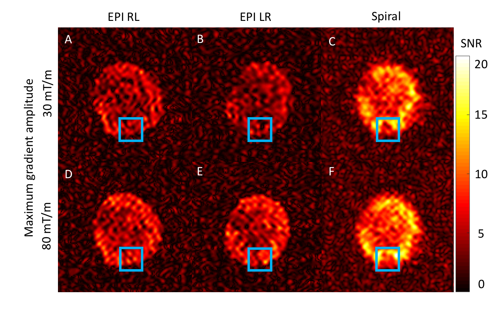
Fig.-3 compares reconstruction results of EPI versus Spiral acquisitions in SNR units. Due to smaller FOV and partial Fourier sampling, EPI trajectories take 40ms while the Spiral trajectory requires 67ms for a maximum gradient amplitude of 30mT/m. At 80mT/m, EPI and Spiral trajectory durations are 23ms and 47ms, respectively. As expected, increasing maximum gradient amplitude results in better image quality (Fig.-3). The highest SNR values are achieved using Spiral acquisitions (Fig.-3C and F) at the expense of effective resolution.

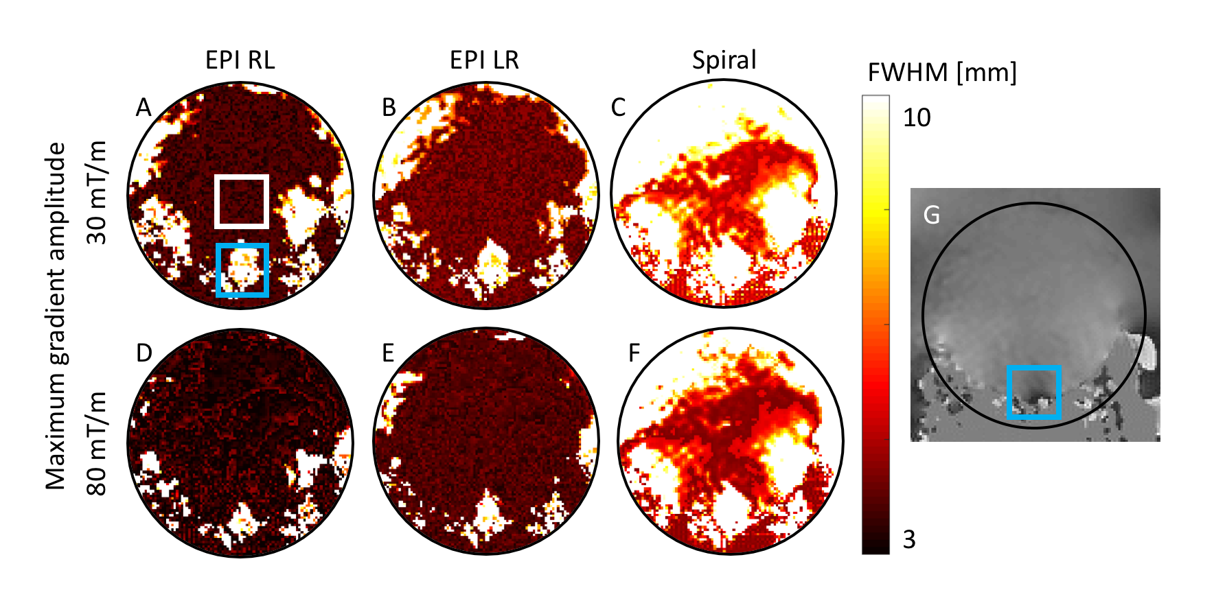
Effective image resolution is analyzed in Fig.-4 demonstrating a general resolution loss relative to the nominal voxel. The mean Full-Width-at-Half-Maximum (FWHM) of the calculated PSFs was determined in an area without strong B0 variations in the blood pool. At 30mT/m the mean FWHM in phase encoding direction is 3.6mm (RL) / 4.1mm (LR) for the EPI trajectory and 5.7mm for the Spiral trajectory. For a maximum gradient amplitude of 80mT/m the respective mean FWHM values are 3.3mm (RL) / 3.8mm (LR) for EPI and 4.8mm for Spiral Imaging. In areas with strong B₀ inhomogeneities these values are vastly increased to 9.1mm (10.7mm) for EPI and to 15.8mm for Spiral Imaging at 30mT/m and to 5.9mm (8.7mm) and 12.6mm at 80mT/m. Especially in regions with 0^th order B₀ offset, Spirals show strong spatial blurring while EPI still allows to delineate local tissue territories.

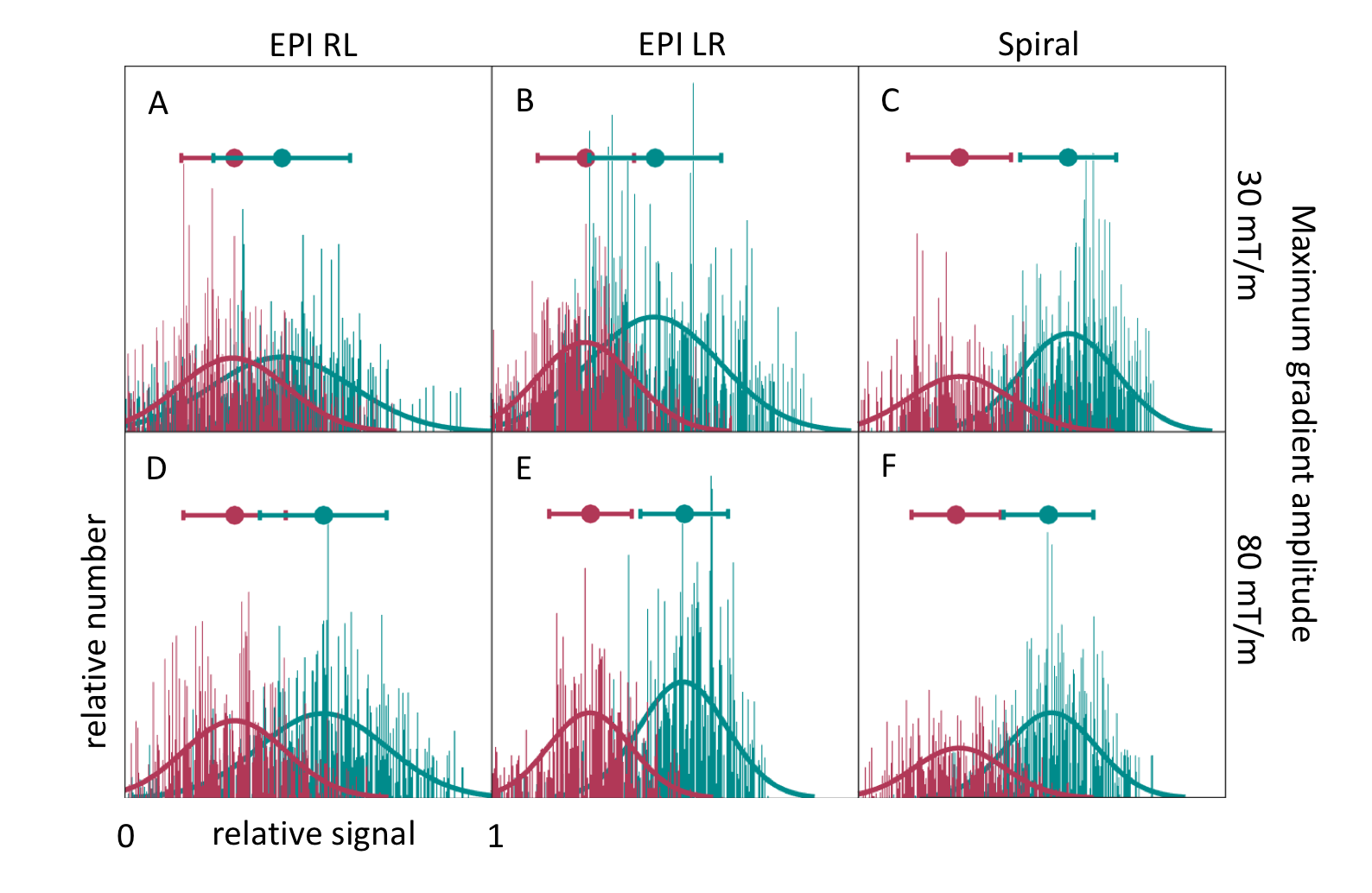
Fig.-5 compares histograms of the signal amplitude within the lesion versus remote myocardium. Mean signal of healthy myocardium is higher than in the lesion, but the difference in mean signal amplitude depends on the utilized trajectory. Spirals yield better detectability of the lesion than EPI trajectories at 30mT/m, however, increasing the maximum gradient amplitude to 80mT/m reduces the relative differences.

Conclusion

Acknowledgements

References

1. Lau JYC, Geraghty BJ, Chen AP, Cunningham CH. Improved tolerance to off-resonance in spectral-spatial EPI of hyperpolarized [1- 13C]pyruvate and metabolites. Magn Reson Med. 2018;100:10158–10 doi: 10.1002/mrm.27086.

2. Miller JJ, Lau AZ, Teh I, et al. Robust and high resolution hyperpolarized metabolic imaging of the rat heart at 7 t with 3d spectral-spatial EPI. Magn Reson Med. 2016;75:1515-1524 doi: 10.1002/mrm.25730.

3. Lau AZ, Chen AP, Hurd RE, Cunningham CH. Spectral–spatial excitation for rapid imaging of DNP compounds. NMR Biomed. 2011;24:988–996 doi: 10.1002/nbm.1743.

4. Park JM, Josan S, Jang T, et al. Volumetric spiral chemical shift imaging of hyperpolarized [2- 13C]pyruvate in a rat C6 glioma model. Magn Reson Med. 2015;75:973-984 doi:10.1002/mrm.25766

5. Durst M, Koellisch U, Frank A, et al. Comparison of acquisition schemes for hyperpolarised 13C imaging. NMR Biomed. 2015;28:715–725 doi: 10.1002/nbm.3301.

6. Segars WP, Sturgeon G, Mendonca S, Grimes J, Tsui BMW. 4D XCAT phantom for multimodality imaging research. Med Phys. 2010;37:4902–4915 doi: 10.1118/1.3480985.

7. Fuetterer M, Busch J, Peereboom SM, et al. Hyperpolarized 13C urea myocardial first-pass perfusion imaging using velocity-selective excitation. J Cardiovasc Magn Reson. 2017;19:46 doi: 10.1186/s12968-017-0364-4.