4224
Fluorine Nanoparticle Quantification in a Mouse Model of Neuroinflammation: Reference-Based Bias Correction for Conventional and Compressed Sensing Reconstructions1Berlin Ultrahigh Field Facility, Max-Delbrück-Center for Molecular Medicine, Berlin, Germany, 2MRI.TOOLS GmbH, Berlin, Germany, 3Experimental and Clinical Research Center (ECRC), Charité Berlin, Berlin, Germany
Synopsis
Fluorine-19 MRI has emerged as a promising tool for in vivo cell tracking, yet low achievable signal-to-noise ratios remain a major challenge. Compressed sensing offers increased sensitivity at the cost of introducing signal intensity bias. We show that at low signal levels the quantification performance of compressed sensing is similar to conventional methods due to signal intensity distribution induced bias effects, which also affect the Fourier reconstruction. To improve quantification results, we propose an intensity correction scheme based on ex vivo reference data.
Introduction
Fluorine-19 MRI has emerged as a promising tool for tracking inflammatory cells in vivo due to its excellent detection specificity. Nonetheless, low achievable signal-to-noise ratios remain a major challenge1. Recently, it was shown that compressed sensing (CS) can help to increase the sensitivity of fluorine MRI2. Negative bias introduced by CS could however compromise the suitability of CS for quantifying the fluorine signal within the cells3. In this study, we investigated the size of these effects for inflammatory cell quantification in the experimental autoimmune encephalomyelitis (EAE) mouse model and propose a signal intensity correction method based on data acquired from ex vivo samplesMethods
All animal experiments were carried out in accordance with local animal welfare guidelines (LaGeSo). EAE was induced in SJL/J mice and perfluoro-15-crown-5-ether rich nanoparticles were administered daily starting on the 5th day after EAE induction4. In vivo data was acquired from three mice on day 13 and 14 after induction and ex vivo data was acquired in tissue phantoms prepared from three different animals. MR experiments were performed on a 9.4T animal scanner (Bruker BioSpin, Ettlingen, Germany). A 3D-RARE protocol was employed for fluorine-19 MRI: TR=800ms, TE=4.4ms, ETL=40, FOV=(45 16 16)mm³, (140 40 50) matrix, 25 repetitions (in vivo), 40 repetitions (ex vivo), 3 averages per repetition. The average of all repetitions was used as reference. A cylindrical cap filled with 2% agarose and 20mM nanoparticles was included for quantification.
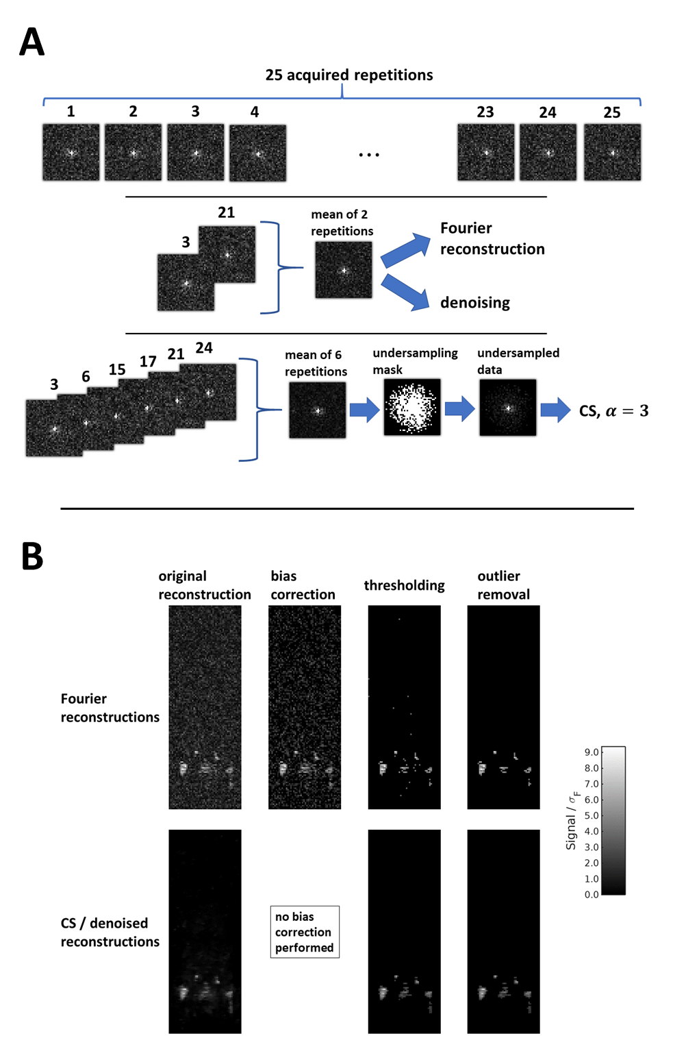
For five different measurement times, fully-sampled and 2 to 5-fold undersampled data were retrospectively sampled (fig.1A). CS and denoised reconstructions were computed using the accelerated alternating direction method of multipliers5 with isotropic total variation and image l1-norm regularization. The deviation of the reconstruction from the measured data was set 97% of the noise level by adjusting the regularization strength. 5 different datasets were generated and reconstructed for each measurement time and method. The Rician noise bias in the conventional Fourier reconstructed magnitude images was corrected as described by Henkelman6. Reconstructions were thresholded at 3.5 (Fourier) or 2 times (denoising and CS) the k-space data noise level. Groups of less than three connected voxels were removed as outliers (fig1B).
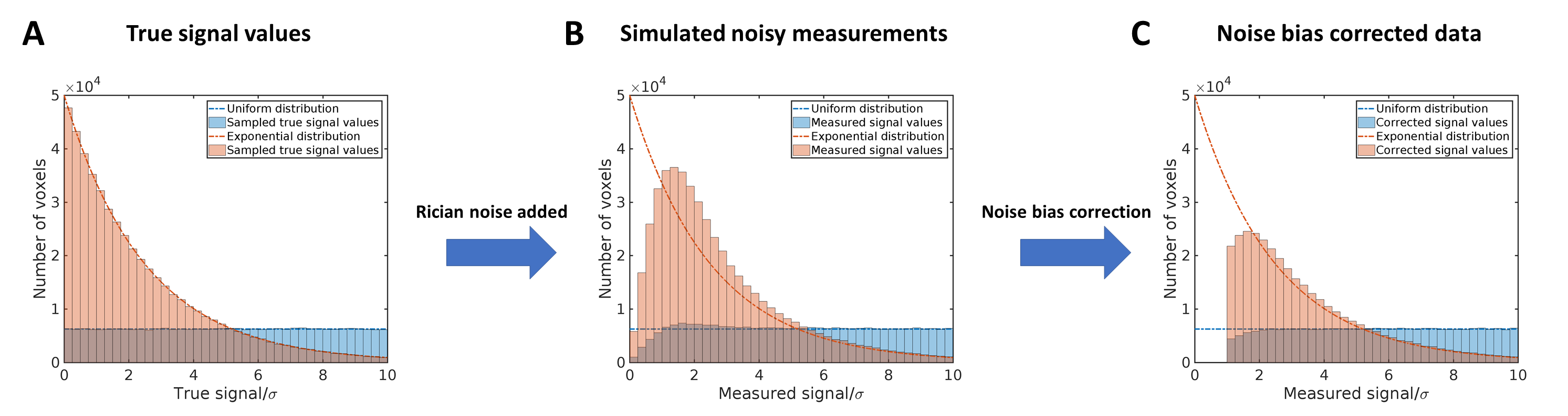
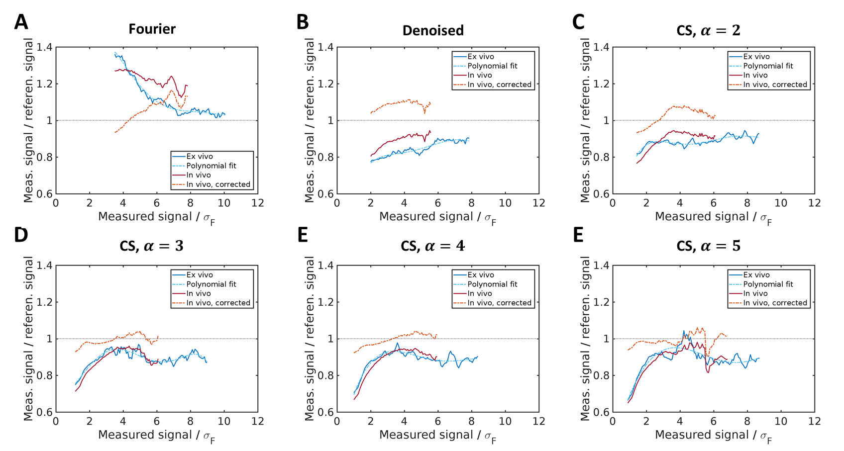
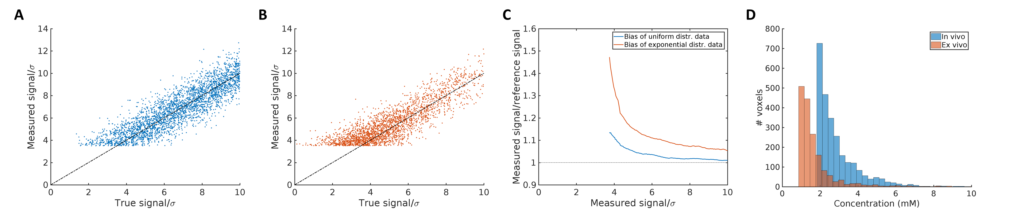
As signal bias depends on the noise level, it was computed for different levels of the measured signal scaled by the noise standard deviation of the Fourier reconstruction at equal scan time σF. Bias correction was performed based on a polynomial fit of the ex vivo data. Simulations testing the interpretation of the observed bias effects were performed as described in fig.2. Reconstructions, simulations and analyses were programmed in MATLAB 2017a (The MathWorks, USA).
Results
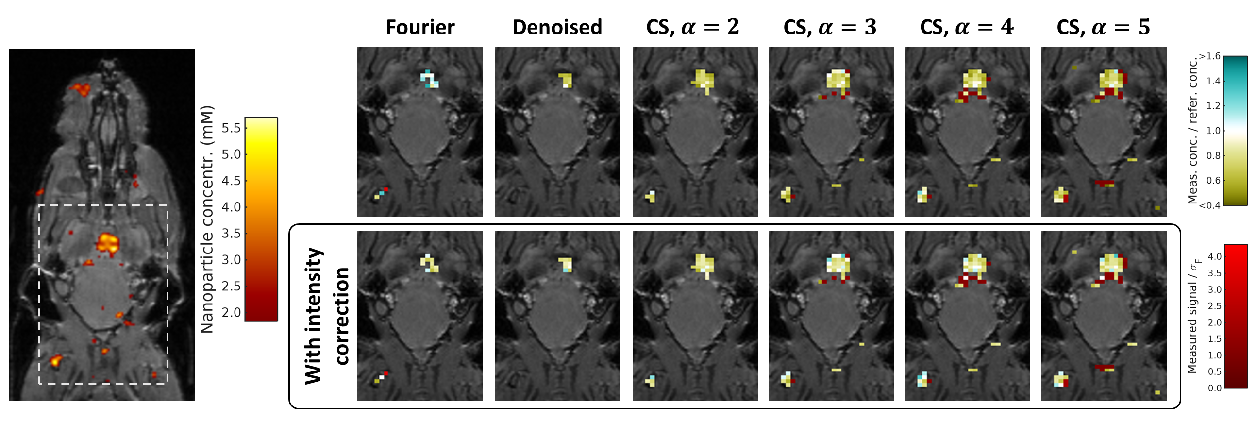
Strong biasing effects were observed close to the detection threshold for all reconstruction methods in both in vivo and ex vivo data (fig.3). While the CS and denoised reconstructions were biased downwards up to 35% close to the signal threshold and by ca. 10% for higher signal levels (fig.3B-F), the Fourier reconstructions overestimated the signal amplitude by as much as 38% (fig.3A). In all cases, the signal bias of the in vivo data could be reduced by the employed correction method, particularly for denoised and CS reconstructions with <10% bias following correction at any signal level (fig.3B-F). The correction was less successful in Fourier reconstructions for signal above . Fig.4 shows corrected reconstructions and a corresponding quantification of nanoparticle concentrations. Simulation results for a uniform sampling distribution showed only slight signal overestimation (fig.5A&C). Fig.5B&C show that a pronounced positive bias is introduced by an exponentially decaying signal intensity distribution. The exponential distribution used is similar to the NP concentration distribution observed in the EAE experiments (fig.5D).Discussion
Our results show that both conventional and CS data are strongly biased at low SNRs. Without correction, CS and conventional reconstructions had similar bias size, albeit in opposite directions. Our proposed reference-based method consistently reduced this bias. While a negative bias of CS reconstructions is expected due to l1-norm minimization, it was partially compensated signal intensity distribution effects. In Fourier reconstructions, these effects introduced a positive bias which could not be corrected as effectively as the CS reconstructions with our method. Our simulations demonstrate that similar effects will occur with any MR data when different signal intensities occur with non-uniform frequency and point towards the need for a robust correction method as proposed here for quantification purposesConclusion
We have shown that accurate nanoparticle quantification in CS reconstructions of fluorine-MRI data can be made possible by employing a correction scheme based on high-quality reference data with similar signal distribution. A sophisticated quantification of the fluorine distribution adds to the benefits of the sensitivity gains of CS.Acknowledgements
This work was supported by two grants of the Deutsche Forschungsgemeinschaft (DFG) to Andreas Pohlmann (DFG PO1869) and Sonia Waiczies (DFG WA2804).References
1. Flögel, U., & Ahrens, E. (2016). Fluorine Magnetic Resonance Imaging. Pan Stanford
2. Starke, L., Waiczies, S., Niendorf, T., Pohlmann, A., (2018). Compressed Sensing Improves Detection of Fluorine-19 Nanoparticles in a Mouse Model of Neuroinflammation, presented at the annual meeting of the ISMRM, Paris, France
3. Hu, S., et al. (2010). 3D compressed sensing for highly accelerated hyperpolarized 13C MRSI with in vivo applications to transgenic mouse models of cancer. Magnetic Resonance in Medicine: An Official Journal of the International Society for Magnetic Resonance in Medicine, 63(2), 312-321.
4. Waiczies, S., Millward, J. M., Starke, L., Delgado, P. R., et al. (2017). Enhanced fluorine-19 MRI sensitivity using a cryogenic radiofrequency probe: technical developments and ex vivo demonstration in a mouse model of neuroinflammation. Scientific Reports, 7(1), 9808.
5. Goldstein, T., O'Donoghue, B., Setzer, S., Baraniuk, R. (2014). Fast alternating direction optimization methods. SIAM Journal on Imaging Sciences, 7(3), 1588-1623.
6. Henkelman, R. M. (1985). Measurement of signal intensities in the presence of noise in MR images. Medical physics, 12(2), 232-233.
Figures