4196
The effect of spatial averaging on dB/dt exposure values for implanted medical devices1The xMR Labs, Department of Physics and Astronomy, University of Western Ontario, London, ON, Canada
Synopsis
We address to what extent the peak dB/dt exposure for active implantable medical devices (AIMDs) desbribed in ISO 10974:2018(E) differs from the spatial average of dB/dt values for devices relevant for testing with realistic spatial extent.
Introduction
The objective of this investigation was to determine the effect that spatial averaging would have on predicted dB/dt values within realistic MRI gradient systems. ISO 10974:2018(E) contains simulated data describing the peak dB/dt values that active implantable medical devices (AIMDs) could be exposed to when within varying compliance volumes within the bore of the MRI scanner. But for devices with realistic spatial extent (e.g. a 5 cm diameter component), the effective dB/dt relevant for testing would be the spatial average dB/dt value over the device. Clearly the average dB/dt value will be smaller than the peak values described in 10974, but the question is, by how much are they decreased? In this abstract we address this question.Methods
The interactions of the example device were investigated over the same range of MRI gradient coils as described in Annex A of 10974, which were designed to represent most possible gradient coil designs that would be found in clinical MRI systems. Three-axis coil sets which corresponded to both 60 cm and 70 cm inner diameter MRI systems were modeled using previously developed and validated methods [1]. They were designed with lengths of: 140, 150, 160, and 170 cm and for each length the size of the imaging region varied over: 35, 40, 45, and 50 cm. For each of these designs, the field produced by all seven axis combinations were separately evaluated, namely GX, GY, GZ, GXY, GXZ, GYZ and GXYZ. A total of 224 different gradient coils were therefore considered in this study.
For each gradient coil design considered, the local dB/dt levels produced were calculated over the surface of a compliance volume within the gradient coil. The grid used in each gradient coil was composed of 777 points, with 21 groups of points from -1 m to 1 m positioned 10 cm apart in the z-direction (along the bore of the gradients) by 37 angular groups of points 10 degrees apart (Figure 1a). The radius of the cylinder was such that when the device was positioned on it, the edge of the device would be located at some ‘compliance radius’. Five different compliance radii were simulated for each gradient axis combination: 10, 15, 20, 25, and 30 cm. In all cases (other than Table 1), the dB/dt values are normalized against the applied gradient slew-rate. To convert the values into dB/dt, they need to be multiplied by the desired single-axis gradient slew-rate.
The device volume was simulated as a 5 cm diameter sphere (Figure 1b). The interior of the device was discretized in a 5 mm rectangular Cartesian grid, with a total of 552 points. The surface of the device was then subdivided more finely, with a number of equally spaced points equal to the number of points on the interior of the device. The surface was more finely subdivided to get more information in the locations that will be closest to the coils of the gradient, where highest dB/dt exposure will occur. The magnetic field was calculated over the device using Biot-Savart methods and the average and peak fields were determined for each location, within each coil.
Results
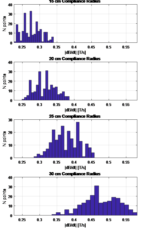
The results obtained across the five different compliance radii are shown in table 1. The dB/dt is broken down into its cartesian components, the average magnitude of the dB/dt, as well as the peak dB/dt for each cartesian component. Figure 2 shows the distribution across the 777 points for a single example coil. Figure 3 shows the distribution for the entire family of coils simulated. Figure 4 shows the peak spatially averaged values across the family of coils broken down by compliance radius and the gradient axis combination.
Discussion
The maximum dB/dt the device experiences increases with compliance radius. For a 5 cm diameter spherical device, across a range of compliance radii from 10 cm to 30 cm radius the highest spatially-averaged dB/dt value that could possibly be experienced across all the combinations of device location and gradient coil design at a slew rate of 200 T/m/s is 116 T/s.Conclusions
How does dB/dt change when we add spatial averaging over a 5 cm sphere? From Table 1, the mean and peak values differ between 2 and 16%. The difference between the peak and mean values increases monotonically, as expected, with compliance radius.Acknowledgements
The authors acknowledge financial support from NSERC and the Ontario Research Fund.
References
1. CT Harris, WB Handler and BA Chronik. Electromagnet Design Allowing Explicit and Simultaneous Control of Minimum Wire Spacing and Field Uniformity. Concepts Magn. Reson., 41B: 120-129 (2012)
Figures
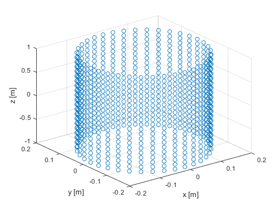
Figure 1a: The calculation grid for the 20 cm compliance radius case. The radius is slightly less than 20 cm so that the 5 cm diameter device with its center at any point on this grid will extend to 20 cm.
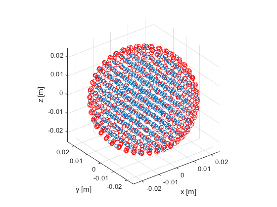
Figure 1b: The 5 cm diameter spherical device used in these simulations, with the points on the surface in red and the points in interior in blue.
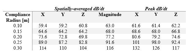
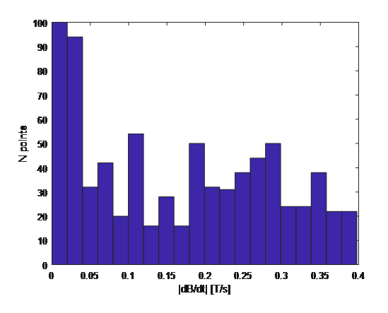
Figure 2: Histogram of dB/dt (magnitude) at all 777 points within one example coil: X gradient of 60 cm diameter, 160 cm length, 45 cm imaging region coil at a 25 cm compliance radius. Values are given as dB/dt per unit Slew-rate of the gradient axes. For a SR-200 T/m/s scanner system, the values above need to be multiplied by 200.
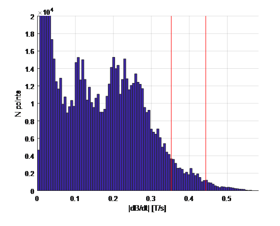
Figure 3: Histogram of all the data across all the coils (and all compliance volumes) with the 95th and 99th percentiles shown (0.352 T/s per SR and 0.443 T/s per SR). Values are given as dB/dt per unit Slew-rate of the gradient axes. For a SR-200 T/m/s scanner system, the values above need to be multiplied by 200.