4183
Comparison of Simulated and Robotically Mapped RF Fields in 64 and 128 MHz Medical Implant Test SystemsKrzysztof Wawrzyn1, Jack Hendriks1, Dereck Gignac1, William B. Handler1, and Blaine A. Chronik1
1The xMR Labs, Department of Physics and Astronomy, Western University, London, ON, Canada
Synopsis
In this work we demonstrate a procedure for the use of a custom-built, semi-automated robotic positioning system to map EM fields in commercially available RF exposure systems and compare the results against FDTD simulations. All field measurements were obtained independently with calibrated E-field or H-field probes. Results show that the robot can effectively operate within the complicated EM environment of the RF exposure platforms with good agreement between simulated and measured results. Future work will continue to improve the techniques discussed here.
INTRODUCTION
Semi-automated robotic mapping of RF exposure in device test platforms is of great value within an ISO 17025-compliant test facility for both verification and validation processes. Establishing and evaluating consistence between measured fields and simulated fields is critical when either is used as part of a medical device testing procedure. In this paper, we show results from proof-of-concept work that demonstrates a procedure for the use of a custom-built, semi-automated robotic positioning system to map electromagnetic fields within and around RF exposure systems and quantitatively compare the results against detailed simulation of those same systems.METHODS
All measurements were performed on two different RF bench top exposure systems, commercially available as “Medical Implant Testing Systems”, or MITS 1.5 and 3.0, corresponding to frequencies of 64 and 128 MHz [1] . The RF exposure parameters for the MITS 1.5 and 3.0 were (respectively): pulse type = sinc2π, duty cycle = 40 %, pulse repetition rate = 1 kHz, polarization = circular 270 & 90 °, frequency = 63.8 & 127.7 MHz, input power = 50 dBm. All field measurements were obtained independently with either a calibrated E-field (EX3DV4) or H-field (H3DV7) RMS probe (EASY4MRI standalone data acquisition system, [1]). The field probes and data collection were fully integrated into a custom built automated robotics system (Figure 1). A 3-axis stepper motor driven gantry robotic field mapping system built in-house was used to gather data. Data collection was taken at points in the unloaded MITS bore at constant spatial increments (3.0 cm) along all directions in an area of XYZ=42×21×42 cm (limit = 50 cm3). A passive algorithm implemented into Labview was used to pursue arbitrary motion objectives and integration with the data acquisition system for data collection. Finite difference time domain (FDTD) computations were carried out using commercially available EMPro 3D EM simulation software [2]. The model was based on the geometry of the physical coils, without lumped elements, using 48 generic ports with sinusoidal excitation at corresponding frequencies. The phase of the signal feeding the source was equal to its azimuthal position and the ports at the same azimuthal position in the two rings were 180-degree out of phase. The simulated field was normalized using a scaling factor determined from a fixed reference H-field location. MATLAB was used to linearly interpolate 3D data onto a 1 mm grid (scatteredInterpolant) and measured data was compared to simulated data using a linear regression model. The reported R-squared values approximate the amount of variation in measurements that is explained by our simulated model.RESULTS AND DISCUSSION
Figure 1 shows a photograph of the automated robotic system with a field sensor at the isocenter of the MITS. A representative 2D plane profile of collected measured and simulated data for MITS 3.0, with percent difference of 4 %, is shown in Figure 2. An example of a line plot through the middle (0 mm) of the 2D profile is shown in Figure 3. The global percent differences in both MITS 1.5 and 3.0 ranged from 3 to 25 % and largely depended on the determined scaling factor. To better quantify the variation of measured to simulated values, a linear regression fit was applied, as shown in the example on Figure 4. Table 1 shows reported R-squared values ranging from 0.83 to 0.97. Lower R-squared values are associated higher variation and may be due to uncertainties in systematic measurement and inaccuracies in the simulation model. Future work will (1) investigate the effect of correcting the correlation with a rigid body transform (2) analyze the accuracy of this method using uncertainty propagation and budgeting, (3) optimize the workflow, (4) compare mapped SAR values within an ASTM phantom [3], and (5) validate the methods against those described in ISO DTS10974 [4].CONCLUSION
In this work, we have presented a protocol and results from proof-of-concept work showing that a semi-automated robotic system can effectively operate within the complicated EM environment of the RF exposure platforms with good agreement between simulated and measured results.Acknowledgements
This work was funded by NSERC, Ontario Research Fund, and the Canadian Foundation for Innovation.References
[1] (ZMT/Speag, Zurich, Switzerland). [2] (Keysight, Santa Rosa, CA). [3] ASTM F2182-11a. [4] ISO/TS 10974:2018(E).Figures
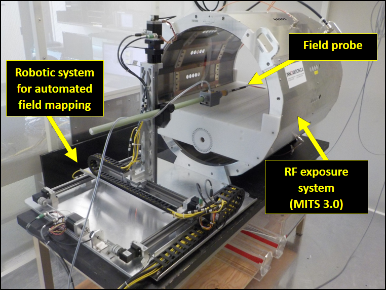
Figure 1: Photograph of the automated robotic system with
a field sensor at the isocenter of the MITS.
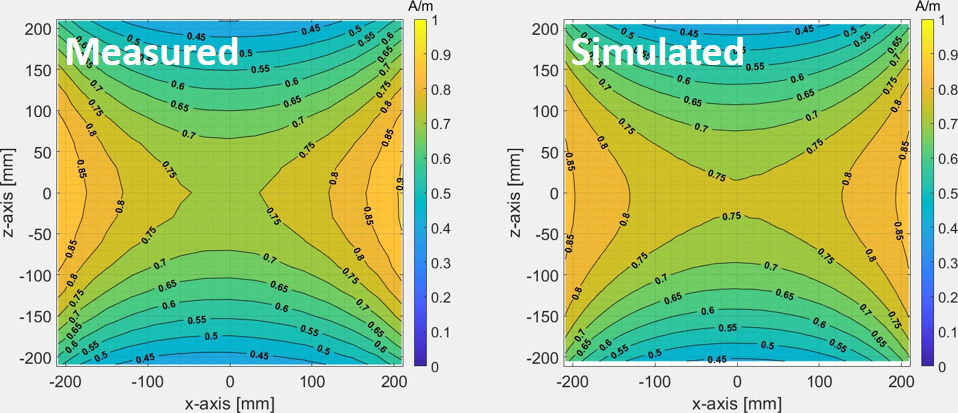
Figure 2: Representative MITS
3.0 2D planes for XZ-axis showing data collected at the geometric coil
isocenter in air (Z-axis = 0 cm). Measured (left) and scaled simulated (right) total
vector magnitude H-field (RMS).
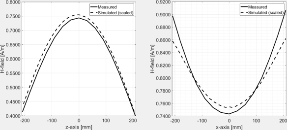
Figure 3: Representative MITS
3.0 line plots produced from a 2D XZ-plane (Figure 1) comparing measured and
simulated H-field. Data points were
taken from dy and dx = 0 mm (left) and dy and dz = 0 mm (right).
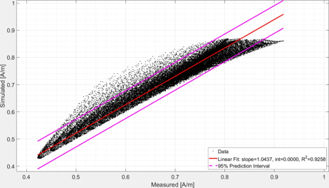
Figure 4: Representative variation of simulated
(y-axis) values with the measured (x-axis) values. Solid red line is a linear
fit to the data. Purple line is 95 %
confidence interval. A summary of
calculated R-squared values are reported in Table 1.
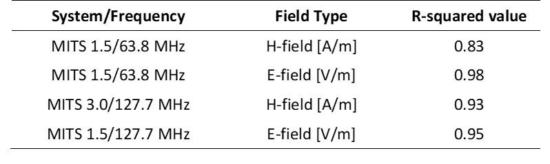
Table 1: Summary of calculated
R-squared values determined by comparing the variation of H-field and E-field
data collected from simulated and measured data in both MITS 1.5 and 3.0.