4165
Effect of helix wire geometry and insulator electrical properties on RF-induced temperature rise and the lead electromagnetic model: a case study1Max Planck Institute for Human Cognitive and Brain Sciences, Leipzig, Germany, 2U.S. FDA, CDRH, Office of Science and Engineering Laboratories, Division of Biomedical Physics, Silver Spring, MD, United States
Synopsis
This case study we investigated RF-induced heating of different helix leads at 127.7 MHz obtained with the lead electromagnetic model (LEM) and direct 3D electromagnetic and thermal co-simulations. A large set of incident electric fields was generated in a phantom by an array of four antennas with varying spatial positions and sources. LEM was validated for predicting temperature in close proximity to the end face of lead tip. However the variance of the fitted values and observed values was rather high for the integral of the power deposition calculated over volume surrounded the lead tip.
Introduction
One of the major components of magnetic resonance imaging safety for patients with an active implantable medical device (AIMD) is the evaluation of in vivo RF-induced heating of tissue near the lead electrode, which can result in tissue damage1-5. One approach to evaluate RF-induced heating is the lead electromagnetic model (LEM) prescribed in Clause#8 of ISO/TS 10974:20186. Using the transfer function (TF) the LEM relates the incident tangential electric field (Etan) along the AIMD lead trajectory to the RF power deposition (P) and temperature rise at a given point in space (ΔTp) due to presence of the lead. In the LEM
$$P = A\cdot | \int_{0}^{L} S(l)\cdot E_{tan}\cdot dl|^{2}$$
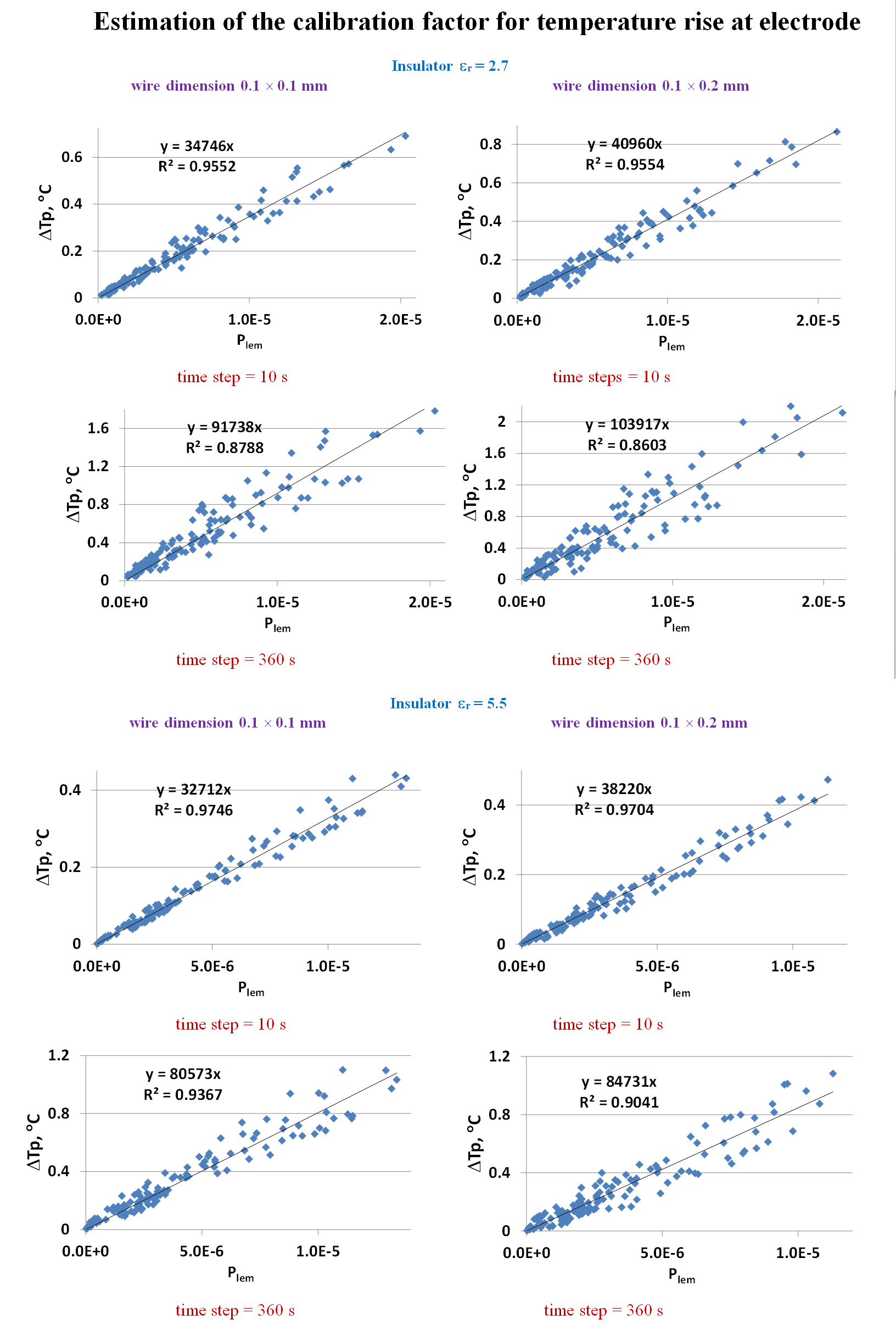
$$\triangle T_{p}= A_{Tp} \cdot | \int_{0}^{L} S(l)\cdot E_{tan}\cdot dl|^{2}$$
where: A and ATp are the calibration factors of the LEM for P and ΔTp, respectively, S(l) is the TF, and L is the lead length. There are a number of different methods that can be used to generate the TF of a lead inside a homogeneous conductive medium, such as piece-wise excitation7 or the reciprocity approach8. The calibration factors A and ATp can be assessed using a linear regression analysis of the results obtained for a set of non-uniform Etan(l). The required Etan(l) characteristics should include the following [6]: regions of high and low incident electric field magnitude, regions of rapidly changing electric field magnitude and phase, and regions where the incident electric field phase changes along the lead at an approximately uniform rate. P and ΔTp obtained from measurement or numerical simulation for each Etan(l) can be combined in sets and plotted against the LEM based prediction
$$ P_{lem}= | \int_{0}^{L} S(l)\cdot E_{tan}\cdot dl|^{2}$$
Plot linear regression provides an estimation of A or ATp as well as R2A and R2ATp, the regression coefficients. If the LEM is validated with low uncertainty, P and ΔTp can be calculated for any Etan(l), including clinically relevant cases.
Methods
Our test objects were four titanium alloy helix wire insulated leads (L=320mm) with an electrode with a diameter of 1.46mm and 10mm in length at one end. At the other end the leads were capped. Two external insulations of 2.5mm in diameter were with relative electrical constant εr={2.7:5.5}. The helixes were 0.1×0.1mm and 0.1×0.2mm rectangular wire with a pitch of 0.35mm and an external diameter of 0.9mm (Figs.1a/b). The leads were positioned in the middle of a box with four antennas located along one side of the box as detailed in8. Box medium electrical properties were similar to blood at 128 MHz (εr=78 and σ = 1.2S/m) (Fig.1c). 120 different Etan(l) were generated by varying the relative antenna positions as well as the amplitude and the phase of each antenna source (Figs.1d). P3D_EM was calculated by integrating the volume loss density (VLD) around the lead tip (Fig.1a). Point VLD values VLD3D_EM were obtained at axial location 1mm from the tip. S(l) was calculated at 161 equidistance points as described in9. The 3D-EM simulations were performed at 127.7MHz using ANSYS HFSS. The 3D temperature distributions at time steps {1,10,60,360,900} seconds for continuous excitation were calculated using the ANSYS NLT package.Results and Discussion
The lead parameter matrix influenced significantly S(l) (Figs.1e) and both calibration factors (Figs.3-4). Thus evaluation of both the TF and the calibration factor should be done for the entire lead parameter matrix. At the lead tip the power deposition and temperature distributions depended significantly on Etan(l) (Fig.2) and the lead parameters. Result variations were evaluated quantitatily using ratios A/AVLD=[0.063:0.098] and ATp/AVLD=[1683:2323] for t=360s as well as R2 of the linear regressions P3D_EM,VLD3D_EM, and ΔTp at 360s versus Plem were in ranges [0.58:0.90], [0.98:1.00] and [0.86:0.94], respectively. Therefore the lead tip power deposition distribution should be evaluated for different Etan(l) if ISO/TS109746 Clause#8 Tier3 approach is applied. For each lead pair (Fig.5) there were subsets of Etan(l) that resulted in higher ΔTp for one or the other lead. Thus to compare different lead designs clinically relevant Etan(l) should be applied.Conclusion
Our case study showed that LEM can be validated for predicting point values of VLD or ΔT at lead tip, despite the fact that power deposition distributions depended not only on lead tip geometry and the surrounding medium but also significantly depended on the lead parameters. Comparison of lead designs using a homogeneous Etan(l) or small set of Etan(l) can result in wrong lead parameter selection in terms of obtaining the lowest ΔTp for most clinically relevant Etan(l).Disclaimer
The mention of commercial products, their sources, or their use in connection with material reported herein is not to be construed as either an actual or suggested endorsement of such products by the Department of Health and Human Services.Acknowledgements
No acknowledgement found.References
[1] L. Panych and B. Madore, “The physics of MRI safety”, J. of Magn. Reson. Imaging, vol. 47, no. 1, pp. 28–432018, 2018.
[2] B. Bhusal et al., “Measurements and simulation of RF heating of implanted stereo-electroencephalography electrodes during MR scans”, MRM, article in press, DOI: 10.1002/mrm.27144, 2018.
[3] P. Bottomley, et al., “Designing passive MRI-safe implantable conducting leads with electrodes”, Medical Physics, vol. 37, no. 7, pp. 3828–3843, 2010.
[4] P. Nordbeck, et al., “Spatial Distribution of RF Induced E-Fields and Implant Heating in MRI”, Magnetic Resonance in Medicine, 60, pp. 312–319, 2008.
[5] Y. Eryaman, et al., “Parallel transmit pulse design for patients with deep brain stimulation implants,” Magnetic Resonance in Medicine, vol. 73, no. 5, pp. 1896–1903, May 2015.
[6] Technical specification ISO/TS 10974, “Assessment of the safety of magnetic resonance imaging for patients with an active implantable medical device”, 2018.
[7] S-M. Park, K. Kamondetdacha, and J. A. Nyenhuis, “Calculation of MRI-induced heating of an implanted medical lead wire with an electric field transfer function”, J. Magn. Reson. Imaging, 26(5), 2007, 1278–1285.
[8] M. Kozlov and W. Kainz,"Lead Electromagnetic Model to Evaluate RF-Induced Heating of a Coax Lead: A Numerical Case Study at 128 MHz", IEEE Journal of Electromagnetics, RF and Microwaves in Medicine and Biology, 2018, DOI: 10.1109/JERM.2018.2865459.
[9] S. Feng, R. Qiang, W. Kainz, and J. Chen, “A technique to evaluate MRI-Induced electric fields at the ends of practical implanted lead,” IEEE Transactions on Microwave Theory and Techniques, 63(1), 2015, 305-313.
Figures