4155

Calculation of the scattered RF field around implants within seconds using a low-rank inverse updating method

Peter R.S. Stijnman^1,2, Janot P. Tokaya¹, Jeroen van Gemert^3,4, Peter R. Luijten¹, Josien P. W. Pluim², Wyger M. Brink⁴, Rob F. Remis³, Cornelis A.T. van den Berg¹, and Alexander J.E. Raaijmakers^1,2

¹Center for Image Sciences, UMC Utrecht, Utrecht, Netherlands, ²Department of Biomedical Engineering, Eindhoven University of Technology, Eindhoven, Netherlands, ³Circuits and Systems, TU Delft, Delft, Netherlands, ⁴Radiology, LUMC, Leiden, Netherlands

Synopsis

Scanning patients that have metallic implants may cause tissue heating. This heating is quantified with electromagnetic simulations. We present an alternative method to quickly compute the electromagnetic response of implants by reducing the problem size using a low-rank inverse updating method. This method requires a pre-computed library of field responses at possible implant locations. Results show computed RF fields that are completely equivalent to full-wave simulations while being 1500 times faster. In particular, computations involving small geometric alterations become faster. This method facilitates rapid field computations and possibly enables online RF- or tier 4 ISO/TS 10974 safety assessment.

Introduction

Scanning patients that have metallic implants with MRI is accompanied with safety risks, one of which is tissue heating through coupling of the implant with radio frequency (RF) fields. To quantify required scanning constraints, electromagnetic simulations of implants are performed. However, these are typically time-consuming. This work presents an alternative and fast method to compute the scattered RF fields around implants by reducing the problem size using a low-rank inverse updating method, which was previously used for dielectric pad optimization.¹

Theory

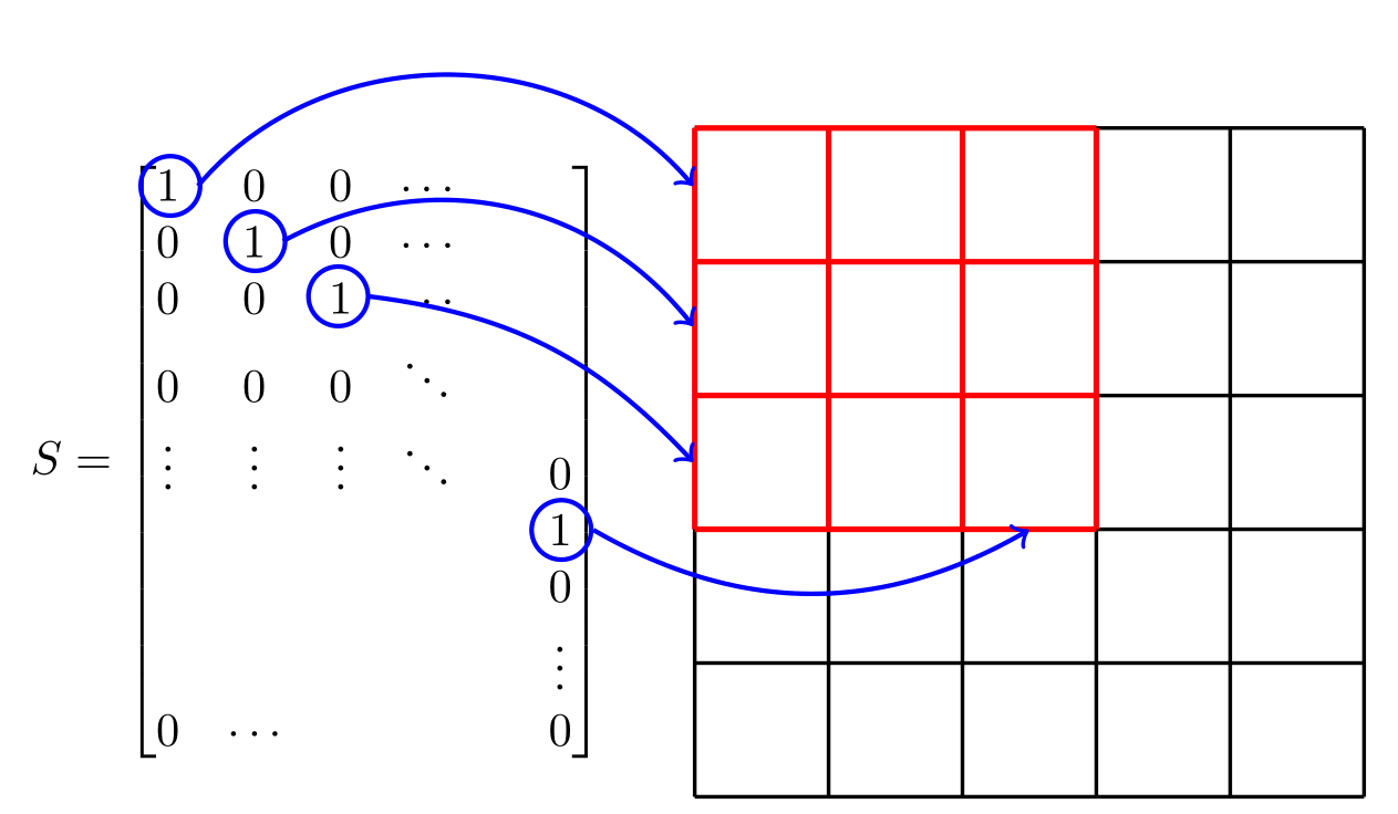
Continuing from¹ we describe the discretized Maxwell equations as$$Af^{bg}=-q.{\quad\quad}(1)$$where $$$A=(D+C)$$$ and $$$D$$$ contains the curl operators and $$$C$$$ contains the geometry and material properties of the human body and the RF coils. Further, $$$f^{bg}$$$ contains the $$$E$$$&$$$H$$$ fields and $$$q$$$ the external current density. Solving for $$$f^{bg}$$$ is impossible through the inversion of $$$A$$$ because it encompasses a large domain. Therefore, numerical methods are used (e.g. FDTD). An implant can be included in the configuration by adding a perturbation matrix $$$C^{imp}$$$, resulting in$$(A+C^{imp})f=-q,{\quad\quad}(2)$$where $$$C^{imp}$$$ is the difference in electrical properties between the implant and the tissue. Compared to the full domain (size $$$N$$$) the implant is only defined on a small domain (size $$$M$$$). Now the support matrix $$$S$$$ is presented (Figure 1), which maps quantities between these domains$$S\tilde{C}^{imp}S^T=C^{imp}.{\quad\quad}(3)$$where $$$\tilde{C}^{imp}$$$ describes a diagonal $$$M{\times}M$$$ matrix. Furthermore, the library matrix$$Z=-A^{-1}S,{\quad\quad}(4)$$is introduced. Every column in this $$$N{\times}M$$$ matrix is the field response for a unitary current density at the corresponding edge in $$$S$$$. This matrix needs to be determined in advance, e.g. by FDTD simulations. Substituting (1),(3),(4) and rewriting (2) we obtain$$f=f^{bg}+Z(I_M-\tilde{C}^{imp}S^TZ)^{-1}\tilde{C}^{imp}S^Tf^{bg}.{\quad\quad}(5)$$using the Sherman-Morrison-Woodbury matrix identity¹ and $$$I_M$$$ is the identity matrix. Given the incident field, $$$f^{bg}$$$, the scattered RF field for an arbitrary implant confined to our small domain can now be found by inverting a matrix of only $$$M{\times}M$$$, which makes the computation feasible and leads to significant acceleration.

(As a matter of fact: $$$(I_M-\tilde{C}^{imp}S^TZ)^{-1}\tilde{C}^{imp}S^T$$$ can be seen as a generalized transfer function/matrix.^2,3)

Methods

The inputs for this method are the RF field distributions without implant and a library matrix. These inputs are computed using an FDTD solver (Sim4Life,ZMT,Zurich,Switzerland). For validation, an additional simulation is performed with the implant present. The resulting field distributions are compared to the fields computed with the presented method. As a proof-of-principle, we used an orthopaedic screw, Figure 2a, placed inside Duke (Virtual family,IT'IS,Switzerland). The location with respect to Duke and the coil are shown in Figures 2b and 2c. The FDTD simulations are done at 128MHz, on a 1mm isotropic grid, using a GPU with a convergence level of -50dB for the incident and total fields and -30dB for the library fields. The inverse computation is performed with Julia⁴ using a conjugate gradient method, with a normal desktop CPU.

Results

Figures 3 and 4 show the resulting $$$E$$$&$$$H$$$ fields respectively. The error for the comparison is defined as$$Err=\frac{f_{FDTD}-f_{inv}}{max(f_{FDTD})}\cdot100\%,{\quad\quad}(6)$$where $$$f_{FDTD/inv}$$$ is substituted for the different field components, $$$f_{FDTD}$$$ are the fields from the FDTD solver, $$$f_{inv}$$$ denotes the fields from the inverse computation. Table 1 shows the maximum errors. The computation of the library took ~15hrs(GPU). The inverse computation took 2.38s whereas the FDTD simulation took 1hr, leading to an acceleration of ~1500.

Discussion

Results show that the presented method provides results that are completely equivalent to the FDTD reference with an acceleration of ~1500. The method is particularly useful for repetitive calculations with small geometric changes, providing great promise for application in tier 4 RF safety assessments (ISO/TS 10974). Furthermore, if the implant geometry could be obtained from prior imaging data, online RF field calculations become feasible. This would result in subject- and situation-specific scanning constraints. The computation time of the presented method depends on the number of edges of the implant but is significantly faster than the FDTD approach if the implant is confined to a relatively small region. However, memory issues still need to be addressed: the library matrix ($$$N{\times}M$$$) for the presented implant already requires 8GB, and grows linearly with the number of edges in the small domain. A potential solution is to undersample the edges that are simulated and use interpolation.

Conclusion

We have shown a new methodology for the assessment of RF field distributions around implants. Using the presented method the RF safety assessment can be done up to 1500 times faster compared to full-wave simulations. The method requires a time-consuming calculation of a so-called library matrix in advance. However, after the library is constructed the RF field enhancement of any arbitrarily shaped and positioned implant, composed of any material, can be computed within seconds.

Acknowledgements

This project is funded by The Netherlands Organisation for Scientific Research (NWO) under project number: 15739.

References

1. J.van Gemert, W.Brink, A. Webb, and R.Remis, “An efficient methodology for the analysis of dielectric shimming materials in magnetic resonance imaging”, IEEE Transactions on Medical Imaging, vol. 36(2), pp 666-673, 2017.

2. J. Tokaya, A.J.E. Raaijmakers, P. Luijten, and C.A.T. van den Berg, "Introduction of the transfer matrix of medical implants enabling unaided MRI assessment of rf safety", Magnetic Resonance in Medicine, vol. 80(6), pp 2771-2784, 2018.

3. S.M. Park, R. Kamondetdacha and J.A. Nyenhuis, "Calculation of MRI-induced heating of an implanted medical lead wire with an electric field transfer function", Journal of Magnetic Resonance Imaging, vol. 26(5), pp 1278-1285, 2007.

4. J. Bezanson, S. Karpinski, V.B. Shah, and A. Edelman, “Julia: A Fast Dynamic Language for Technical Computing”,arXiv, 2012.

Figures

A representation of the $$$S$$$ matrix for a two-dimensional grid. The left shows the values inside the support matrix for the corresponding edges in the grid on the right. The red edges define the small domain while the red plus the black edges define the large domain. The blue arrows indicate to which edge in the grid each '1' corresponds. The red edges indicate the possible edges an implant could occupy.

The geometry and location of the passive implant inside Duke. The left, (a), figure shows the model of the screw used inside Duke. The middle, (b), figure shows a transverse slice of Duke inside the birdcage coil showing the position of the screw. The right, (c), figure shows a sagittal slice of Duke inside the birdcage coil showing the position of the screw.

The magnitude of the electric field components. The three rows show the magnitude of the $$$E_{x,y,z}$$$ components respectively. The first column shows the electric fields computed by the FDTD method. The second column shows the results of the computation done with the presented methodology. The last column shows the error percentage, from 0 to 1%, as computed by Equation (6).

The magnitude of the magnetic field components. The three rows show the magnitude of the $$$H_{x,y,z}$$$ components respectively. The first column shows the magnetic fields computed by the FDTD method. The second column shows the results of the computation done with the presented methodology. The last column shows the error percentage, from 0 to 1%, as computed by Equation (6).

Maximum error percentage in $$$E$$$ and $$$H$$$ fields as computed by Equation (6) for the entire domain. The error is scaled by the maximum value in the field, rather than the local field value. Otherwise small deviations in regions where the actual fields are also very small (e.g. inside the implant) would result in large error values although these deviations are of minor concern.

Proc. Intl. Soc. Mag. Reson. Med. 27 (2019)

4155