4028
Deep Quantitative Susceptibility Mapping by combined Background Field Removal and Dipole Inversion1Department of Neurology, Medical University of Graz, Graz, Austria, 2Centre for Advanced Imaging, The University of Queensland, Brisbane, Australia
Synopsis
Deep learning based on u-shaped architectures has been successfully used as a means for the dipole inversion crucial to Quantitative Susceptibility Mapping (QSM). In the present work we propose a novel deep regression network by stacking two u-shaped networks and consequently both, the background field removal and the dipole inversion can be performed in a single feed forward network architecture. Based on learning the theoretical forward model using synthetic data examples, we show a proof-of-concept for solving the background field problem and dipole inversion in a single end-to-end trained network using in vivo Magnetic Resonance Imaging (MRI) data.
Introduction
In vivo mapping of magnetic susceptibility has gained broad interest in medicine because it yields relevant information on biological tissue properties, predominantly myelin, iron and calcium. QSM is a novel method which calculates magnetic susceptibility from MRI gradient echo phase data by solving an ill-posed field-to-source-inversion problem. After MRI acquisition the phase images are analytically unwrapped, the background field is removed and finally the dipole inversion is deconvolved, nowadays mainly by the use of iterative regularization methods [1, 2]. Recently, deep learning approaches have been used for solving the dipole inversion by either the usage of synthetic data to learn the forward problem (deepQSM [3]) or by using multiple orientation data (QSMnet [4]). However, these methods require a background field removal by SHARP, PDF or LBV [5]. Therefore we propose a novel deep regression network which does not only perform the dipole inversion but additionally removes the background field from the input data in a single feed forward network architecture.Methodology
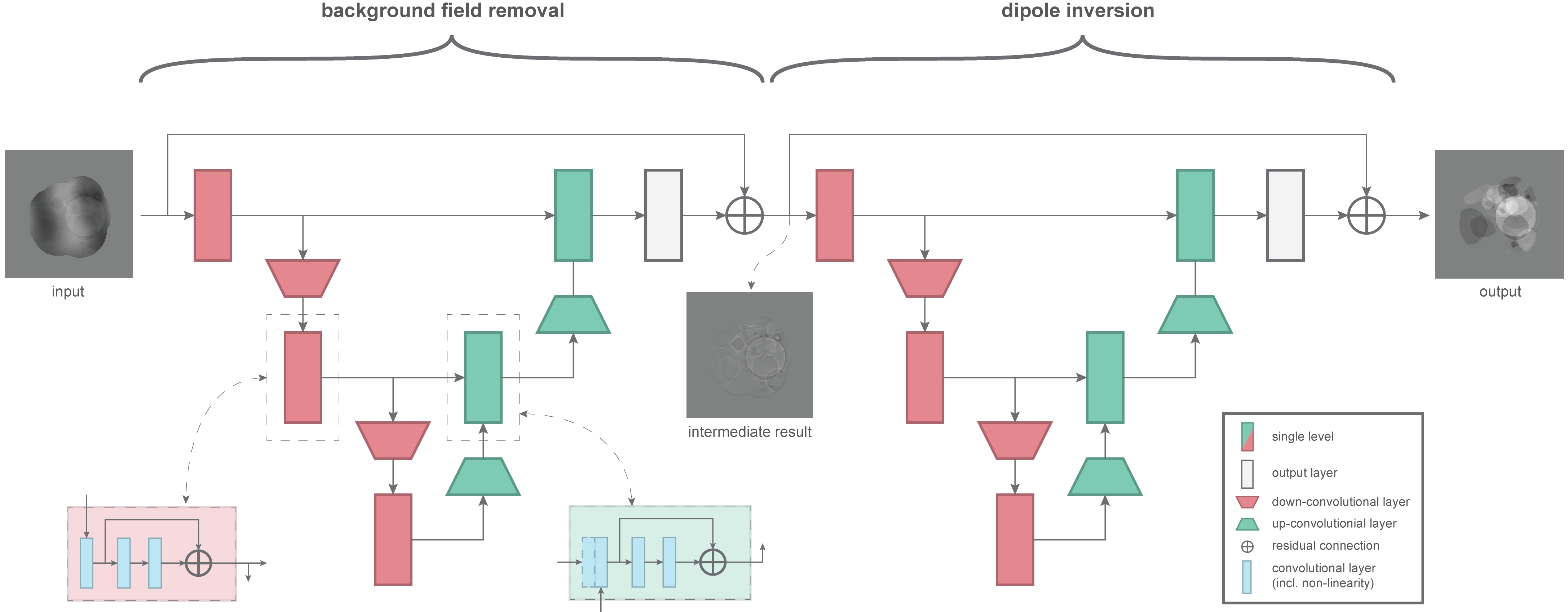
Network architecture. Based on the architecture proposed for deepQSM [3], we present a Fully Convolutional Network (FCN) [7], that stacks two u-shaped sub-networks [8]. Those u-shaped sub-networks are trained to perform the background field removal and the dipole inversion, respectively (cf. Figure 1 for details). Each u-shaped sub-network involves two symmetric parts, an encoding and a decoding part. In the first part those networks encode relevant information from the given input into a set of high-level feature maps, while in the second part the generated feature maps are then decoded to the desired output. An important aspect of u-shaped networks is the use of skip connections, that connect layers in the encoding part with the corresponding layers in the decoding part. Those connections allow to preserve high frequency information. At the end of each u-shaped network we use a convolutional layer to map to one output channel. Hence we obtain an intermediate result, where the background field is removed, after the first u-shaped network, and a final susceptibility result at the end of the network.
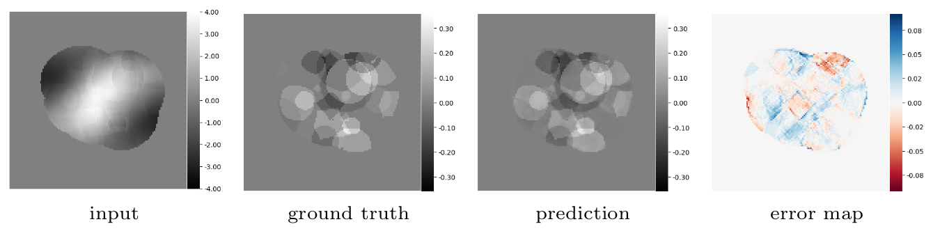
Synthetic data generation and network training. In order to train the proposed network a large amount of training data is needed for supervised training. For this purpose we created a synthetic dataset where geometric objects were randomly positioned in space and assigned a certain susceptibility to mimic anatomic regions (cf. Figure 2). Those ground truth susceptibility maps were then convolved using a dipole kernel in the Fourier domain. For our current purpose we generated 1100 random samples, with a size of 128 × 128 × 128. The entire dataset is further split up into a training set of 1000 samples and test set of 100 samples. We use data augmentation to train models invariant to predefined data deformations, including additive random low frequency background fields and high frequency image acquisition noise. In order to train the proposed network we use the Tensorflow framework [9], where we chose Adam [10] to optimize the L1 loss between the intermediate result and the input data without the background field, and between the final output and the given ground truth susceptibility map. We trained the model end-to-end for approximately 32k iterations, where we used a batch size of 2.
Experimental Results
Synthetic evaluation. Figure 2 provides an evaluation based on synthetic data from the generated test set. Note, that the obtained predictions are visually nearly indistinguishable from the ground truth data, which shows that the network is able to perform the given task.
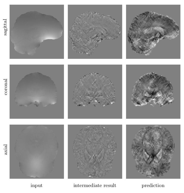
In vivo MRI evaluation. Figure 3 shows predicted QSM images and intermediate images based on MRI gradient echo phase data from the 2016 QSM reconstruction challenge [2]. We can observe that the network is able to generalize to this unseen data.
Discussion and Conclusion
In this work, we proposed a QSM algorithm based on deep neural networks. The expected function of our network is to invert the magnetic dipole kernel convolution by simultaneously being invariant to low frequency background fields. Our presented results demonstrate that it is indeed possible to train a network to perform this task in an end-to-end manner. We also showed that our trained model is able to generalize to real world data from in vivo MRI scans. Although our predicted susceptibility maps still include some reconstruction artifacts, we expect to further improve the reconstruction quality by training a larger version of the proposed architecture. Finally we also eliminated the hurdle of acquiring a large labeled real world dataset for supervised training by training our model merely on synthetic data.Acknowledgements
This research was supported by a NVIDIA GPU hardware grant.References
[1] Y. Wang and T. Liu, “Quantitative susceptibility mapping (qsm): Decoding mri data for a tissue magnetic biomarker,” Magnetic Resonance in Medicine, vol. 73,01 2015.
[2] C. Langkammer, F. Schweser, K. Shmueli, C. Kames, X. Li, L. Guo, C. Milovic,J. Kim, H. Wei, K. Bredies, S. Buch, Y. Guo, Z. Liu, J. Meineke, A. Rauscher,J. P. Marques, and B. Bilgic, “Quantitative susceptibility mapping: Report from the 2016 reconstruction challenge,” Magnetic Resonance in Medicine, vol. 79,no. 3, pp. 1661–1673.
[3] K. G. B. Rasmussen, M. J. Kristensen, R. G. Blendal, L. R. Ostergaard,M. Plocharski, K. O’Brien, C. Langkammer, A. Janke, M. Barth, and S. Boll-mann, “Deep qsm - using deep learning to solve the dipole inversion for mri susceptibility mapping,” bioRxiv, 2018.
[4] J. Yoon, E. Gong, I. Chatnuntawech, B. Bilgic, J. Lee, W. Jung, J. Ko, H. Jung,K. Setsompop, G. Zaharchuk, E. Y. Kim, J. Pauly, and J. Lee, “Quantitative susceptibility mapping using deep neural network: Qsmnet,” NeuroImage, vol. 179,pp. 199 – 206, 2018.
[5] F. Schweser, S. D. Robinson, L. d. Rochefort, W. Li, and K. Bredies, “An illustrated comparison of processing methods for phase MRI and QSM: removal of background field contributions from sources outside the region of interest,” NMR in Biomedicine, Oct. 2016.
[6] A. L. Maas, A. Y. Hannun, and A. Y. Ng, “Rectifier nonlinearities improve neural network acoustic models,” in in ICML Workshop on Deep Learning for Audio,Speech and Language Processing, 2013.
[7] J. Long, E. Shelhamer, and T. Darrell, “Fully convolutional networks for semantic segmentation,” in 2015 IEEE Conference on Computer Vision and Pattern Recognition (CVPR), pp. 3431–3440, June 2015.
[8] O. Ronneberger, P. Fischer, and T. Brox, “U-net: Convolutional networks for biomedical image segmentation,” CoRR, vol. abs/1505.04597, 2015.
[9] M. Abadi, A. Agarwal, P. Barham, E. Brevdo, Z. Chen, C. Citro, G. S. Corrado, A. Davis, J. Dean, M. Devin, S. Ghemawat, I. Goodfellow, A. Harp, G. Irving,M. Isard, Y. Jia, R. Jozefowicz, L. Kaiser, M. Kudlur, J. Levenberg, D. Mané,R. Monga, S. Moore, D. Murray, C. Olah, M. Schuster, J. Shlens, B. Steiner,I. Sutskever, K. Talwar, P. Tucker, V. Vanhoucke, V. Vasudevan, F. Viégas,O. Vinyals, P. Warden, M. Wattenberg, M. Wicke, Y. Yu, and X. Zheng, “TensorFlow: Large-scale machine learning on heterogeneous systems,” 2015. Software available from tensorflow.org.
[10] D. P. Kingma and J. Ba, “Adam: A method for stochastic optimization,” CoRR,vol. abs/1412.6980, 2014.
Figures