INTRODUCTION

Separation of different CEST effects in the Z-spectrum is challenging especially at low field strengths where amide, amine and NOE peaks coalesce with each other or with the water peak. While successful Lorentzian peak separation was shown at ultra-high fields [1], the coalescence and broad peaks are relatively hard to isolate at 3T [2]. However, we could show that this peak information is still in the 3T spectra and can be extracted with a deep learning approach by training with 9.4T human brain target data [3]. The performance and optimization of this deepCEST approach is investigated herein for different network architectures and trainings.

METHODS

Highly-resolved Z-spectra of the same volunteers were acquired by 3D-snapshot CEST MRI [4] at 3T (53 offsets, 1.7x1.7x3mm) and 9.4T (95 offsets, 1.5x1.5x3mm) and coregistered. 9.4T-Z-spectra were fitted by a multi-Lorentzian model, which yields in each voxel a vector of optimized multi-Lorentzian parameters popt containing spectral position, width and amplitude of each CEST-Lorentzian. The data was acquired from three healthy subjects as well as one brain tumor patient after written informed consent. A feedforward neural network (FFNN) as well as several convolutional neural networks (CNNs) were trained: CNN 1 (two convolutional + maximum pooling layers with window size 9,32 and 64 filters respectively), CNN 2 (residual block architecture [5], two convolution window 3 layers inside the blocks, while every 3 blocks, the filter size was doubled, starting at 32 filters. When the filter size was doubled, convolution with stride 2 halved the spectral resolution. In accordance to [6], identity connections were used around the residual blocks), CNN 3 (as CNN 2 but doubled filter sizes and an additional layer, 64, 128, 192 filters, decreasing convolution window of 9, 7 and 5). All networks were trained to predict 9.4T amide and NOE amplitudes from 3T Z-spectra of healthy subject and on the tumor patient data as untrained test set. The influence of the amount of training data on the models was tested by comparing the training when using different number of subjects. CNNs were not given any information about neighboring voxels as to learn inference solely from Z-spectra to the Lorentzian fit of the spectrum; thus the feature of convolutions to include and encode neighborhood information is focused on spectral neighborhood herein.

RESULTS

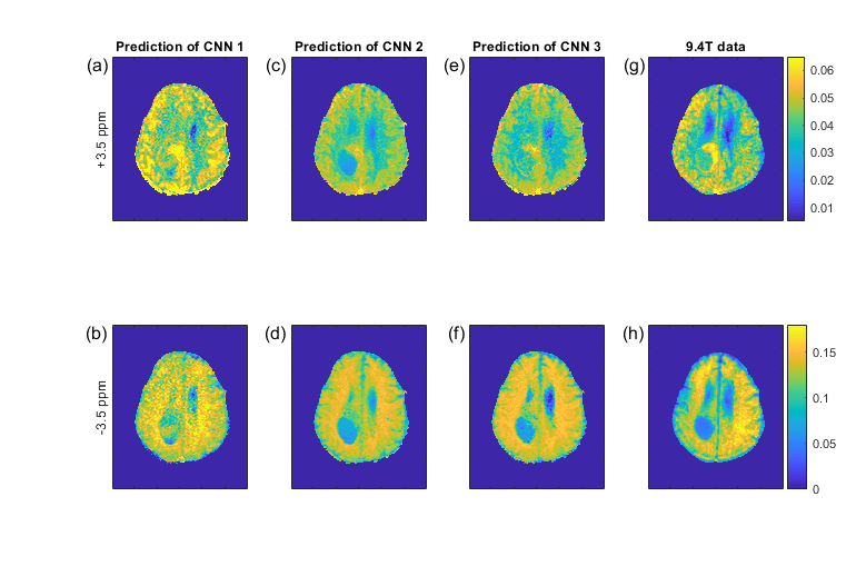
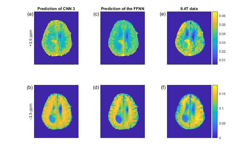
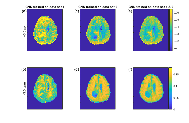
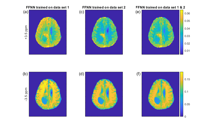
Figure 1 shows the pseudo 9.4T CEST contrast predictions from 3T data in the tumor patient for different CNN architectures together with the measured 9.4T CEST maps. Network optimization is a necessary step as prediction performance strongly depends on the network architecture (Figure 1); from left to right, the number of free parameters of the models increase as well as their prediction performance. Figure 2 compares the prediction of CNN 3 in the left column to the prediction of the FFNN (center column) and the real 9.4T data (right column). The optimized CNN shows similar predictions as the previously used FFNN, yet the FFNN shows a better denoising ability, leading to smoother results in general. The CNN shows some more heterogeneous features in the tumor area that are also visible in the real data. The prediction performance of the CNNs depends on the training data, but can be improved by combining training data sets (Figure 3). This is a general property of deep learning approaches and was found as well for the FFNN (Figure 4).

DISCUSSION

Herein we investigated different network architectures for the deepCEST approach. Although we expected that CNNs perform better than FFNNs due to their equivariance to feature positions in the input, a fairly straightforward FFNN can learn the B0 corrected data even better so far. Also, the wide range of prediction quality is an indicator for the improvements that can still be achieved by further tuning the CNN networks until their performance is expected to surpass that of the so-far best FFNN. It was surprising that the sophisticated ResNet-Architecture [5,6], which has high performance in image recognition, speech and language processing, performed worse than the straightforward approach of stacking convolutional and pooling layers when translated to this task of convolution in the spectral domain. We showed that our networks learned to predict previously unseen brain data and were capable of accurately displaying tumor regions, which emphasizes the generalization capability of our approach.

CONCLUSION

Machine learning might be a powerful tool for CEST data processing and could bring the benefits and insights of the few ultra-high field sites to a broad clinical use. At the same time, optimization and adaption of network architecture is an important step to improve deepCEST prediction performance.

Acknowledgements

The financial support of the Max Planck Society, German Research Foundation (DFG, grant ZA 814/2-1), and European Union’s Horizon 2020 research and innovation programme (Grant Agreement No. 667510) is gratefully acknowledged.