4001
Producing a Synthetic Magnetization Transfer Reference Volume with T1 Maps Acquired using a Different Pulse Sequence: Practical Considerations.1Centre for Addiction and Mental Health (CAMH), Toronto, ON, Canada, 2Psychiatry, University of Toronto, Toronto, ON, Canada
Synopsis
Macromolecular proton fraction (MPF) mapping can be achieved using only two acquired volumes, one with and one without a magnetization transfer (MT) pulse, in addition to T1, B1 and B0 maps. Further scan time reduction is possible if the T1 and B1 maps required for MPF computations are used to generate a synthetic reference image, eliminating the reference image acquisition. This has been shown to work when the images used to generate T1 were acquired from the same sequence and parameters as the MT. We investigate if we can use a different sequence with a calibration to achieve this.
Introduction
The Magnetization Transfer (MT) effect indirectly probes the presence of macromolecules. An MT ratio map is the most practical, albeit somewhat arbitrary, measurement of the MT effect that measures the relative change in signal between two volumes: one acquired with an MT saturation pulse at a frequency offset, Δ, (MTΔ) and a reference image (MT0) acquired identically but without the MT pulse. A more accurate, quantitative map of the macromolecular proton fraction (MPF)2-5, shown to correlate with myelin6, can be generated from a two-pool model and is expected to yield more interpretable results. Traditionally, MPF requires several MTΔ volumes and is too time-consuming for clinical applications2,3,5. Recent work shows that an accurate MPF can be obtained using a single, optimal MTΔ2,4. Furthermore, a faster implementation has been proposed3 where the required T1 and B1 maps for MPF are used to generate a synthetic MT0 (synMT0). In that work, the T1 maps used to compute synMT0 are obtained using a two-point (S1, S2) variable flip angle (VFA)7 approach, where (S1, S2) are acquired using the same sequence (spoiled gradient echo, SPGR), resolution and timing scan parameters as those used for MTΔ. Given strict timing constraints for the MTΔ acquistion, imposed by increasingly restrictive SAR limitations and the required MT pulse, imposing the same constraints on (S1, S2) is not optimal for T1 accuracy nor scanning efficiency.
T1 mapping has been previously optimized and calibrated8,9 with a method that relies on the fast SPGR sequence, FSPGR, which uses a shortened RF pulse, allows for SENSE10-like acceleration and is not compatible with MT saturation experiments due to SAR limitations. The goal of this work is to investigate if we can create a synMT0 using FSPGR-based T1 maps, that can be used with an SPGR-based MTΔ for MPF measurements. The T1 maps are produced at 1 mm3 in ~10min scan time, which is approximately equal to the scan time for a single MTΔ acquisition at (1.6 mm)3. In particular, we seek to find a subject-independent calibration factor, f, that can be used to scale synMT0 when it has been generated from an FSPGR-based T1 map. We present a calibration method and discuss practical considerations (e.g., error propagation).
Method
The SPGR signal, S, can be described by Eq.1 as:
$$ S=\frac{S0 \cdot (1-E1) \cdot sin(B1 \cdot \alpha)} {(1-E1\cdot cos(B1 \cdot \alpha)} $$
where E1=exp(-TR/T1), B1 is the flip angle (α) error due to B1+ and S0=ξ·σsp ·Scoil · PD · exp(-TE/T2), where Scoil is the coil sensitivity, PD is proton density, σsp is a scaling term that reflects poor spoiling signal offset and ξ is a scanner-dependent scaling of the signal. Accurate synMT0, requires accurate S0. If the spatially dependent contributions of Scoil, PD and T2 are accurate, a scaling factor, f, can be determined to calibrate for differences in ξ and σsp across acquisitions. S0 can be computed from either S1(α=3°) or S2(α=14°), given T1 and B1 maps via Eq.1. The result should differ by a constant scaling: S0(S1)/S0(S2)=1/σsp, resulting from α-dependent poor RF spoiling of S2 but not on S19. Here, we aim to compute synMT0 to within a scaling factor at best because we expect ξ to differ across sequences adn acquisition parameters: FSPGR (ξF ) and the SPGR (ξS). We propose to correct for multiplicative factors (ξ·σsp) by f: i.e., if we use S0(S1), we expect the f to account for ξF , ξS and σsp(αMT), where αMT is the excitation α used for MTΔ .
Four healthy volunteers are scanned on a 3T MR scanner (GE, MR750) as per institutional IRB. Simulations are used to assess the sensitivity of S0 computations to errors in B1 and/or T1. Using calibrated T1 and B1 maps8-10 produces unbiased maps thus we compute T1 and B1 stability errors from repeat measurements on one subject. We perform a calibration (Table1) to determine if synMT0 and MT0 are related through a simple scaling.
Results
Fig.2 shows that S0 is not very sensitive to T1 errors and somewhat sensitive to B1 errors. Furthermore, significant errors in T1 and B1 would produce a spatially dependent S0 error (dependent on local true T1 and B1 values). Repeat measurements show relatively low T1 and B1 errors translate to even lower S0 errors, independent of true T1 and B1 values (Fig.3). Fig.4 demonstrates the calibration steps on a single subject and the successful calibration of synMT0 with f=(12.6) -1. Fig.5 shows the same f can be used for the other subjects.Conclusions
We show that a synthetic MT reference image can be generated using T1 maps computed from signal of a different sequence than MTΔ as long as a proper calibration is performed.Acknowledgements
No acknowledgement found.References
- Wolff SD, Balaban RS. Magnetization transfer contrast (MTC) and tissue water proton relaxation in vivo. Magnetic Resonance in Medicine 1989;10(1):135-144.
- Yarnykh VL. Fast macromolecular proton fraction mapping from a single off-resonance magnetization transfer measurement. Magnetic Resonance in Medicine 2012;68(1):166-178.
- Yarnykh VL. Time-efficient, high-resolution, whole brain three-dimensional macromolecular proton fraction mapping. Magnetic Resonance in Medicine 2016;75(5):2100-2106.
- Trujillo P, Summers PE, Smith AK, et al. Pool size ratio of the substantia nigra in Parkinson's disease derived from two different quantitative magnetization transfer approaches. Neuroradiology 2017;59(12):1251-1263.
- Yarnykh VL. Pulsed Z-spectroscopic imaging of cross-relaxation parameters in tissues for human MRI: Theory and clinical applications. Magnetic Resonance in Medicine 2002;47(5):929-939.
- Khodanovich MY, Sorokina IV, Glazacheva VY, et al. Histological validation of fast macromolecular proton fraction mapping as a quantitative myelin imaging method in the cuprizone demyelination model. Scientific Reports 2017;7.
- Wang HZ, Riederer SJ, Lee JN. OPTIMIZING THE PRECISION IN T1 RELAXATION ESTIMATION USING LIMITED FLIP ANGLES. Magnetic Resonance in Medicine 1987;5(5):399-416.
- Chavez S, Stanisz GJ. A novel method for simultaneous 3D B1 and T1 mapping: the method of slopes (MoS). Nmr in Biomedicine 2012;25(9).
- Chavez S. Assessing B1 map errors in vivo: measuring stability and absolute accuracy despite the lack of gold standard. International Society of Magnetic Resonance in Medicine (ISMRM). Paris, France; 2018. p. 2269.
- Chavez S. Calibrating variable flip angle (VFA)-based T1 maps: when and why a simple scaling factor is justified. International Society of Magnetic Resonance in Medicine (ISMRM). Paris, France; 2018. p. 537.
- Pruessmann KP, Weiger M, Scheidegger MB, Boesiger P. SENSE: Sensitivity encoding for fast MRI. Magnetic Resonance in Medicine 1999;42(5).
Figures
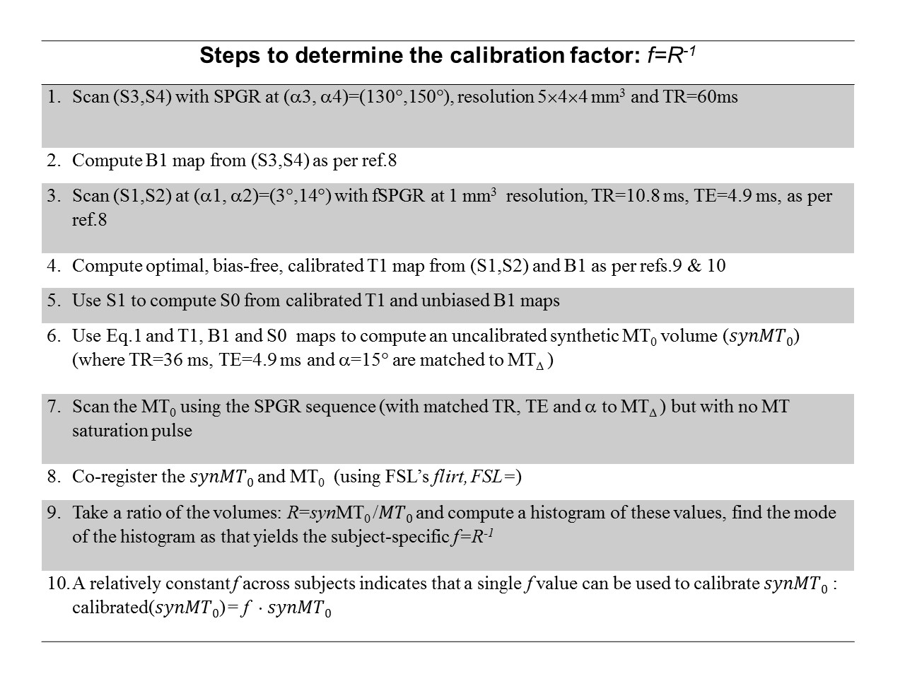
Table 1
Steps 1-9 are performed on each subject, i, to determine if a subject-specific constant calibration factor can be found: $$$ f_{i}=(\frac{MT_0}{synMT_0})_i $$$. If $$$ f_i $$$ values are consistent across subjects, an average can be used as the sought calibration factor for synMT0 : $$$ f= ave(f_i) $$$. In practice, we work with $$$ R=f^{-1} $$$ instead because $$$ R>1 $$$ in our case.
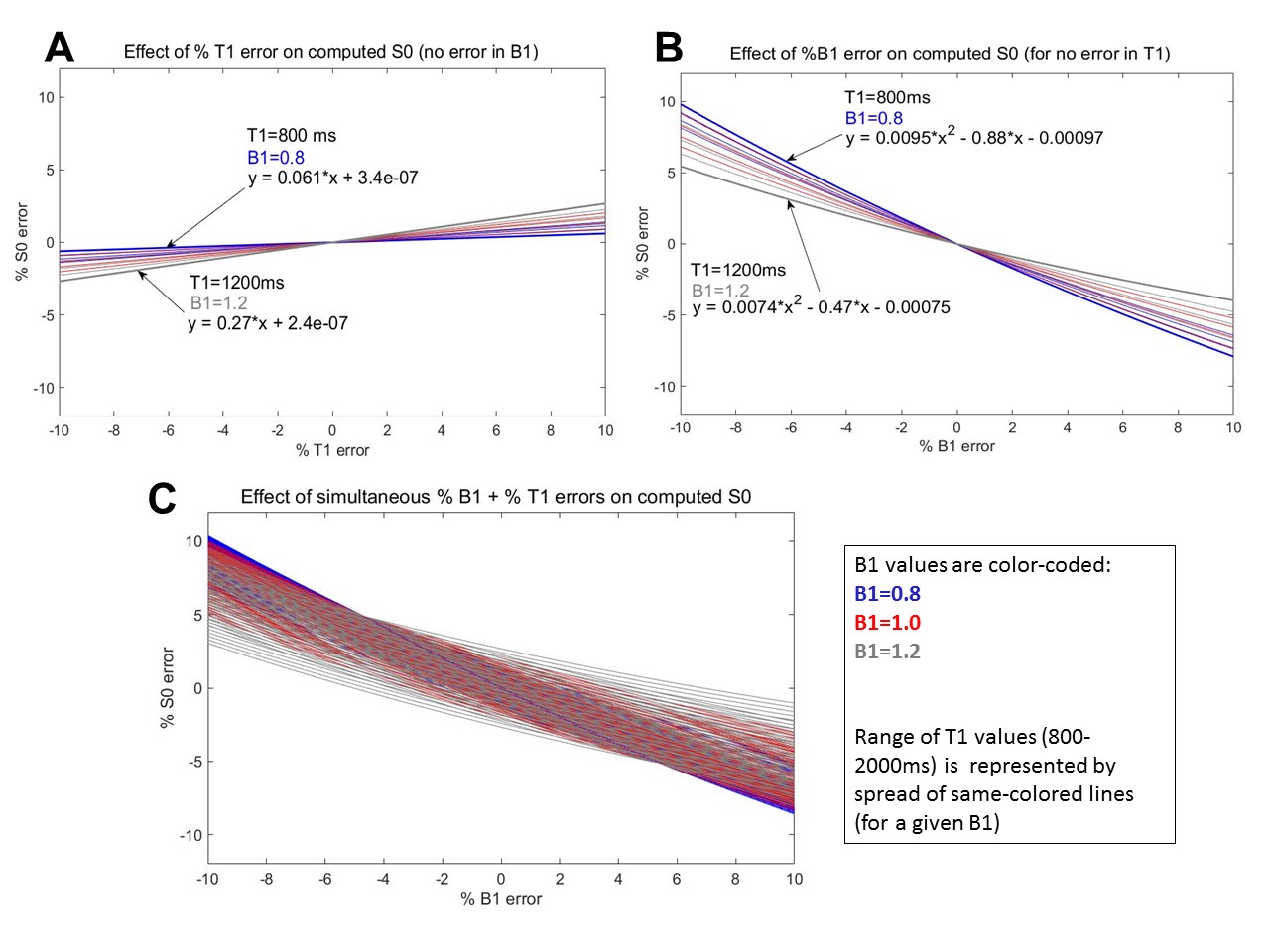
Figure 1
Simulations are used to study error propagation. For S0=10, S1 is computed from (B1,T1,S0) for a range of expected B1 and T1 values: B1= (0.8-1.2) and T1=(800-2000 ms). Relative errors ($$$ \pm 10\%$$$) are introduced step-wise as ε=(0.9:0.02:1.1). A. For each (B1,T1) set, step-wise ε gives T1'=εT1 and S0'(B1,T1',S0) and the relative S0 error =100%· (S0-S0')/S0. B. Same as A but for B1 C. B1' and T1' are computed for all combinations of ε values. Simultaneous B1 and T1 errors cause a spread of the curves in B; the relative S0 error remains within 10%.
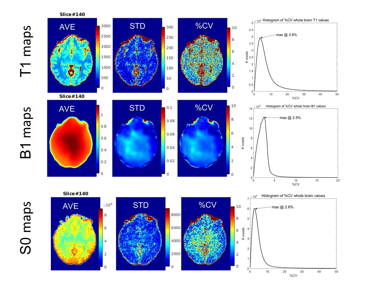
Figure 2
Demonstration of the errors associated with repeat measurements: Subjects were scanned for (S1,S2,S3,S4) 3x, yielding 3 sets of independent T1, B1 and S0(S1) maps. Average (AVE), standard deviations (STD) and coefficients of variation (CV=STD*100%/AVE) are computed voxel-wise for each resulting map. Figures show representative slices and histograms show whole brain values. Smooth, low resolution B1 maps have small errors which propagate into both the T1 and S0 maps. Higher T1 errors occur in the CSF but S0 maps are not highly affected. No tissue contrast in STD(S0) indicates no significant tissue-specific errors from T1 or S0 maps.
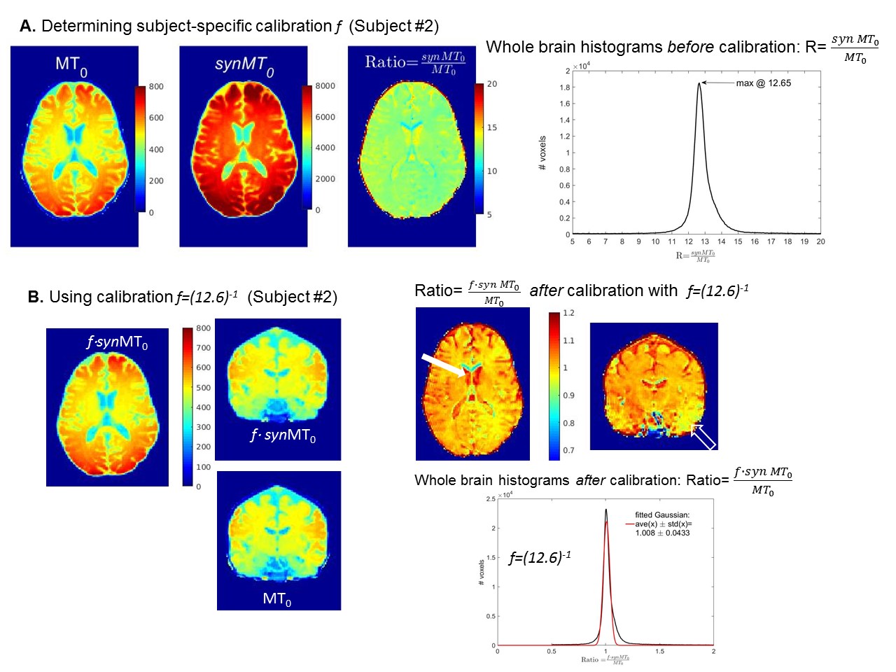
Figure 3
A subject-specific $$$ f_{2}=R_{2}^{-1}$$$ was determined as per Table 1 for subject #2. A shows the relative signal offset between MT0 and synMT0. A histogram of whole brain R values gives the subject-specific scaling: the mode = $$$ R_{2}=12.65 $$$. B shows the result when synMT0 is calibrated by $$$ f=(12.6)^{-1} $$$ (compare axial slice with MT0 in A). The ratio=$$$ f $$$ · synMT0/MT0 demonstrates that the calibration works well (shown by the representative figure and whole brain histogram of ratio values centered at 1.008). White arrows indicate areas of $$$MT_0$$$ discrepancy in regions with CSF (filled) and B0 inhomogeneity (hollow).
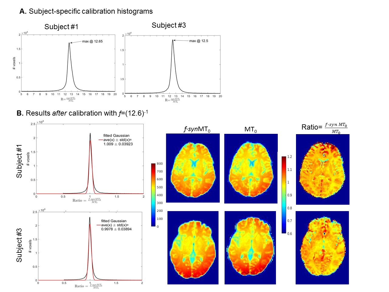
Figure 4
Determination of the subject specific $$$f_i$$$ are shown in A: $$$f_{1}= (12.65)^{-1} $$$ and $$$ f_{3}=(12.5)^{-1} $$$ . B. Shows that using an average $$$f=ave(12.65,12.65,12.5)^{-1}=(12.6)^{-1}$$$, results in a good calibration of synMT0 for subjects #1 and #3 as well (given by the whole brain ratio histograms centered at 1.009 and .9978 for subjects #1 and #3 ,respectively).