3982
Neural network for fast quantitative magnetization transfer imaging1Korea Advanced Institute of Science and Technology, Daejeon, Korea, Republic of, 2Seoul National University Hospital, Seoul, Korea, Republic of
Synopsis
Quantitative magnetization transfer (
INTRODUCTION
The quantitative magnetization transfer (qMT) imaging provides quantitative information of the magnetization exchange between the macromolecular pool and the free water pool [1]. However, the long scan time is one of the obstacles for qMT imaging to be routinely used in clinics. Recently, deep learning approaches are suggested to solve many issues of biomedical imaging [2,3]. In this study, a neural network is proposed for the acceleration of qMT imaging by taking 4 MT images as input and predicting the full 12 MT images as output. This will reduce the acquisition time by a factor of 3 and hence increase chances of clinical translation and decrease undesired artifacts such as motion artifacts. The network was tested on conventional qMT and inter-slice qMT datasets [4].METHODS
All datasets were obtained from 7 healthy volunteers using a Siemens 3T Tim Trio system (Siemens Medical Solutions, Erlangen, Germany). Balanced SSFP was used as readout for both conventional and inter-slice qMT with scan parameters of TE=2.275ms, TR=4.55ms, matrix size=128´128, slice thickness=5mm, FOV=220´220 mm², and number of slices=1 (conventional) and 25 (inter-slice). T1 and T2 maps were obtained by inversion recovery bSSFP and multi-echo spin echo, respectively. For both qMT imaging methods, total 12 MT images were acquired at 6 off-resonance frequencies (2, 3, 5, 9, 15, 25kHz) with two MT saturation RF flip angles (30°, 75°). Since MT effects at 25 kHz off-resonance were negligible, the images of 25 kHz off-resonance were considered as MT free images, by which all the data was normalized.
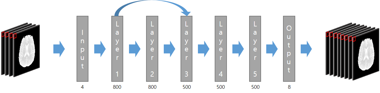
The network was trained to take 4 MT images as input and to predict the 8 MT images at the remaining off-resonance frequencies as output. The network was composed of 6 fully-connected layers with the sigmoid activation function. A dense connection [5] was applied between layer1 and layer3 (Fig. 1).
For training, Adam optimizer [6] with learning rate 0.001 was used to reduce the mean squared error (MSE) with scaling factor 0.01. Seven-fold cross-validation was used to validate the results. Early stopping was applied after 100 epochs for conventional qMT and 2000 epochs for inter-slice qMT. To train the conventional qMT data, the network was pre-trained with the inter-slice data to compensate for the small data size.
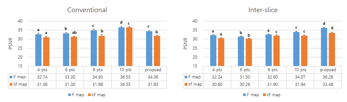
The outputs from the various input choices were compared to choose the best frequencies for the 4 input. The two MT images from 25 kHz offset were always included for the data normalization and the remaining one off-resonance frequency for each FA was searched. The qMT fitting was conducted to find the exchange rate (kf) and the pool fraction (F) for the data from the deep learning networks and also using only 4, 6, 8 and 10 MT images in the conventional way with no deep learning, through the database approach described in Kim. J-W et al. [4]. The qMT fitting applied to the original 12 MT images was used as ground truth. The performance was evaluated by peak signal-to-noise ratio (PSNR), structural similarity (SSIM) and normalized root mean squared error (NRMSE).
RESULTS and DISCUSSION
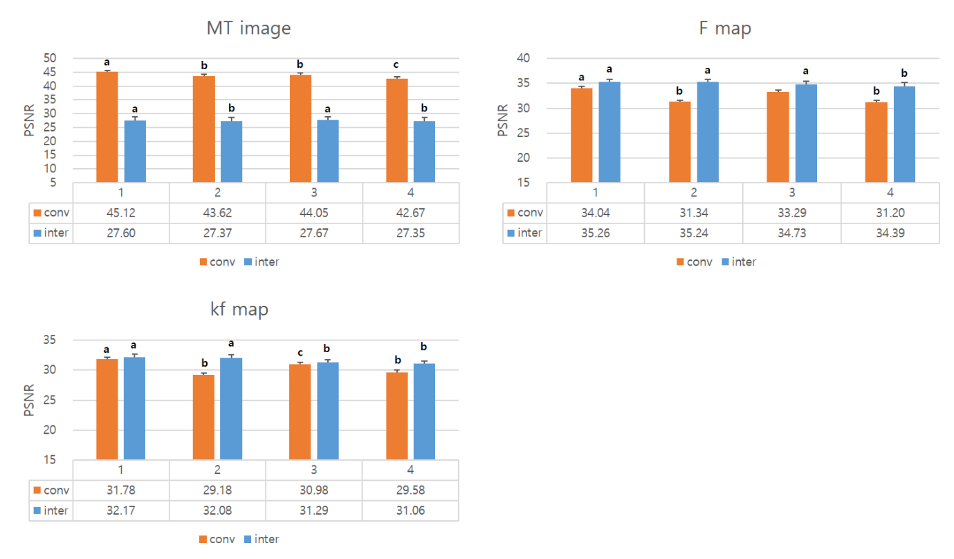
For the comparison of input frequency choice, the set of 2 kHz and 25 kHz showed the best results for both flip angles (Fig. 2), so this frequency set was used in the remaining experiments.
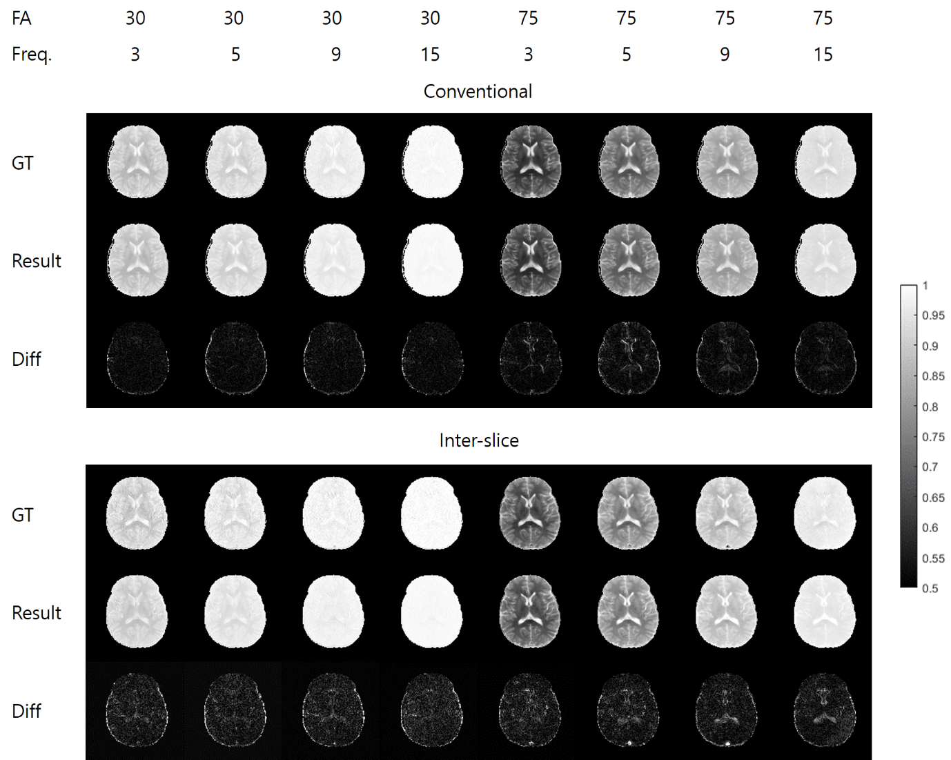
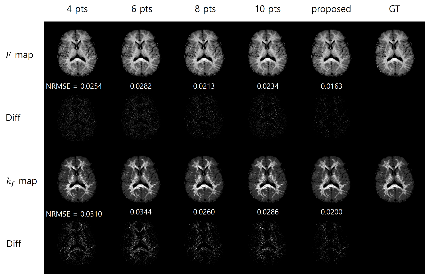
Figures 3 and 4 are the predicted MT images from a representative subject. PSNR / SSIM / NRMSE for the conventional and inter-slice qMT datasets were $$$45.2\pm1.8$$$ / $$$0.9936\pm0.0006$$$ / $$$0.0056\pm0.0011$$$ and $$$39.4\pm1.3$$$ / $$$0.9801\pm0.0029$$$ / $$$0.0110\pm0.0017$$$, respectively. Network for conventional qMT showed better performance than that for the inter-slice qMT, presumably due to higher SNR of the images. Figures 4 and 5 show the qMT fitting results. For the conventional qMT, the network trained with the 4 input MT images showed performance comparable to those of the 8-MT images processed in the conventional way with no deep learning. On the other hand, for the inter-slice qMT the network trained with the 4 input MT images showed higher performance than all the conventional approach including the case of the 10 MT images. The difference in performance of the deep learning networks between the conventional and inter-slice qMT maps might be related to data size used for training.
CONCLUSION
The proposed deep learning networks could reduce the scan time by a factor of 3 with relatively high SSIM and PSNR and low NRMSE, indicating qMT results of the networks close to those of the ground truth. Further studies are necessary for the network to be improved by training with larger data from various subjects including patients.Acknowledgements
No acknowledgement found.References
1. HENKELMAN, R. Mark, et al. Quantitative interpretation of magnetization transfer. Magnetic resonance in medicine, 1993, 29.6: 759-766. 2. RONNEBERGER, Olaf; FISCHER, Philipp; BROX, Thomas. U-net: Convolutional networks for biomedical image segmentation. In: International Conference on Medical image computing and computer-assisted intervention. Springer, Cham, 2015. p. 234-241. 3. KIM, Ki Hwan; DO, Won‐Joon; PARK, Sung‐Hong. Improving resolution of MR images with an adversarial network incorporating images with different contrast. Medical physics, 2018. 4. Kim. J-W, et al. Rapid whole brain qMT imaging with inter-slice MT effects and database-driven fitting approach. 26th Annual Meeting, ISMRM 2018; Program number: 2754 5. HUANG, Gao, et al. Densely Connected Convolutional Networks. In: CVPR. 2017. p. 3. 6. KINGMA, Diederik P.; BA, Jimmy. Adam: A method for stochastic optimization. arXiv preprint arXiv:1412.6980, 2014.Figures