3968

Magnetic resonance shear wave elastography using transient acoustic radiation force excitations and sinusoidal displacement encoding

Lorne W. Hofstetter¹, Henrik Odéen¹, Bradley D. Bolster, Jr.², Allison Payne¹, and Dennis L. Parker¹

¹Department of Radiology and Imaging Sciences, University of Utah, Salt Lake City, UT, United States, ²Siemens Healthcare, Salt Lake City, UT, United States

Synopsis

A novel elastography approach that uses sinusoidal motion encoding gradients to encode the displacement time-history following a single transient acoustic radiation force excitation is presented. This technique may be particularly well suited for performing elastography before, during, and after MR-guided focused ultrasound treatments since the same device used for therapy is used as an excitation source for elastography.

Introduction

MR-guided focused ultrasound (MRgFUS) is a completely non-invasive ablation technique that is used for a number of clinical indications. The mechanical properties of ablated tissue often differ from those of healthy tissue^1-3. Evaluating tissue stiffness during MR-guided focused ultrasound (MRgFUS) procedures could complement current treatment monitoring and assessment methods. While magnetic resonance elastography (MRE) enables in-vivo determination of tissue shear stiffness, adding the external driver required for mechanical excitation to an already complex MRgFUS setup may not be feasible. In this work we present a novel elastography approach that uses the MRgFUS transducer to generate transient mechanical excitations and sinusoidal motion encoding gradients (MEGs) to encode the resulting displacement time-history in a way that enables the tissue shear wave speed to be calculated. Since the therapy device is used as the excitation source for elastography, this method could be readily integrated into the workflow of MRgFUS therapies.

Theory

Using the shear component of the Green’s function of Bercoff et al.⁴ the mechanical shear waves generated by the acoustic radiation force (ARF) from a focused ultrasound (FUS) transducer can be modeled as:$$d(\vec{r},t)=f(\vec{r},t)\otimes g_s(\vec{r},t)$$where $$$d(\vec{r},t)$$$ is the displacement along the FUS propagation direction, $$$f(\vec{r},t)$$$ is the FUS generated forcing distribution, $$$\vec{r}$$$ is the in-plane radial position relative to the FUS beam axis, $$$r=|\vec{r}|$$$, $$$\otimes$$$ is the multi-dimensional convolution in both $$$\vec{r}$$$ and time $$$t$$$ and$$g_s(\vec{r},t)=\frac{1}{4\pi\rho{c_{s}}}\frac{1}{\sqrt{2\pi\nu_{s}{t}}}\frac{1}{r}\cdot{e^{\frac{-(c_st-r)^2}{2 \nu_{s} t}}}$$ is the Green’s function for the $$$y=0$$$ plane where $$$c_s$$$ is the shear wave speed, $$$\nu_s$$$ is the kinematic shear viscosity, and $$$\rho$$$ is the tissue density. The time history of this transient tissue displacement can be encoded in MR image phase using an MEG, $$$G(t)$$$, whose direction is parallel to the FUS beam. The accrued MR image phase can be written:$$\phi(\vec{r})=\gamma\int_0^T G(t){\cdot}d(\vec{r},t)dt$$where the MEG is executed on the interval $$$[0,T]$$$. If two phase images $$$\phi_c$$$ and $$$\phi_s$$$ are acquired using gradient waveform shapes $$$G_c=A{cos(\omega{t})}$$$ and $$$G_s=A{sin(\omega{t})}$$$, respectively, where $$$A$$$ is the peak gradient amplitude and $$$\omega$$$ is the frequency of the oscillatory waveform, a synthetic phase image can be constructed$$Z=\phi_c+i\phi_s=\gamma{A}\int_0^Td(\vec{r},t){\cdot}{e^{i\omega{t}}}dt.$$ For a reasonably compact displacement packet, $$$d(\vec{r},t)$$$, $$$Z$$$ becomes:$$Z\propto{e^{i \omega t_a}}$$where the arrival time at position $$$r$$$ is$$t_a=\int_0^r\frac{dr'}{c_s(r')}.$$ The shear wave speed map can be readily calculated from the two equations above:$$c_s(\vec{r})=\frac{\omega}{\frac{d}{dr}(\angle{Z})}$$where $$$\angle{Z}$$$ is the complex argument of $$$Z$$$. The above equation provides an elegant approach to interrogating the shear stiffness (or shear wave speed) in settings where FUS generated ARF generated excitations are possible.

Methods

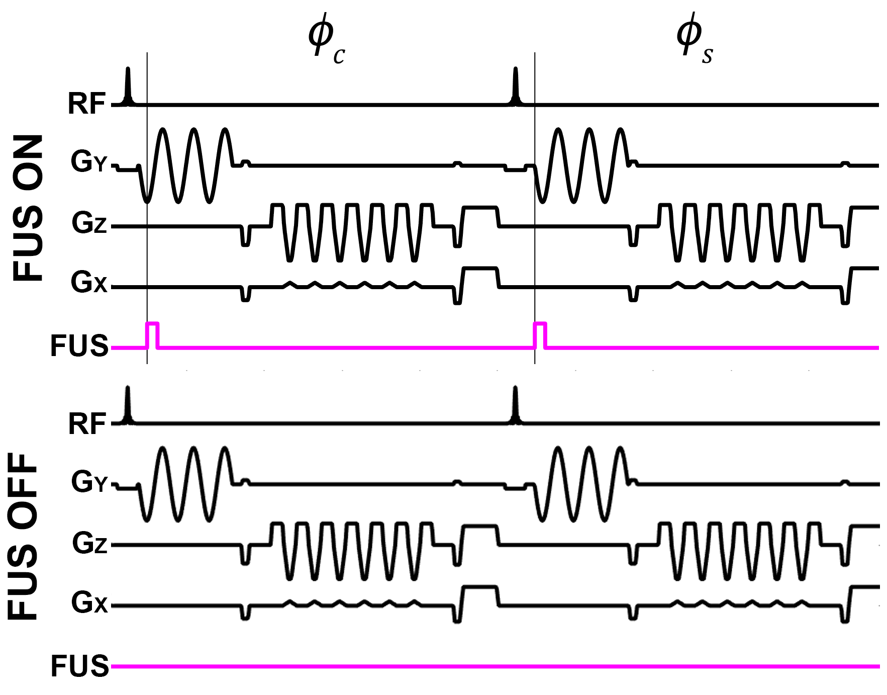
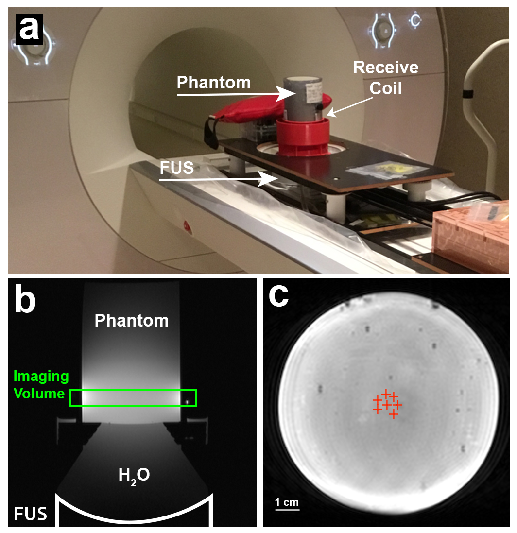
A segmented EPI pulse sequence with sinusoidal motion encoding gradients was implemented on a 3T MRI scanner (MAGNETOM Prisma^Fit, Siemens Healthcare, Erlangen, DE) and phase images $$$\phi_c$$$ and $$$\phi_s$$$ were acquired in a homogeneous gelatin phantom. Using a preclinical MRgFUS system (256-element, 950 kHz frequency, 13 cm focal length, Image Guided Therapy, Inc.), one ARF pulse (106 acoustic Watts, 2 ms duration) was triggered per repetition time (TR) interval. The FUS excitation location was varied every other TR to interrogate a slightly different region in the phantom. This interleaving scheme was repeated until k-space for each imaging volume corresponding to each spatial ARF location was fully acquired. In total the phase images $$$\phi_c$$$ and $$$\phi_s$$$ were acquired for 8 imaging volumes (7 with FUS on, and one reference without FUS). Figure 1 depicts the pulse sequence and FUS timing scheme. Figure 2 depicts the experimental setup and ARF excitation locations. MR measurement parameters were: TE|TR = 31|51 ms, FA=23°, ETL=7, Matrix 128x133x12, 1x1x5 mm resolution, MEG amplitude|period|#cycles = 60 mT/m|6 ms|3 cycles. Shear wave speed maps for each ARF location were generated using the equation for $$$c_s(\vec{r})$$$. A composite shear wave speed map was generated by combining measurements at the 7 ARF positions.

Results

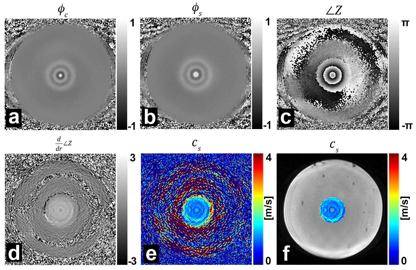
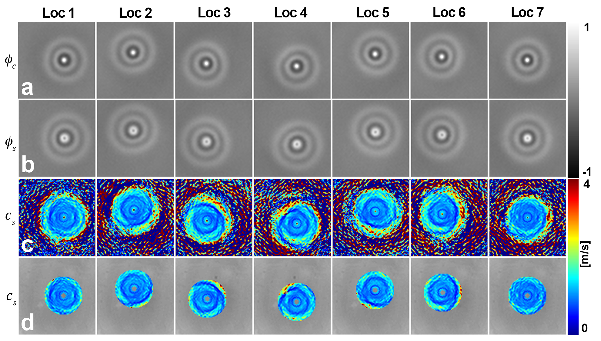
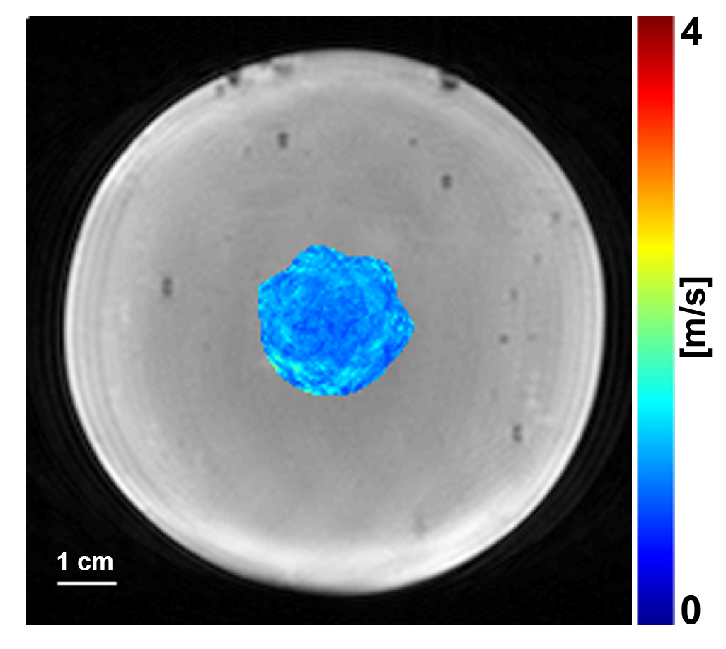
Figure 3 shows the intermediate quantities and calculated shear wave speed map for a single ARF location. The phase and shear wave speed maps for the 7 ARF locations are depicted in Figure 4. Figure 5 shows the composite map where measured mean shear wave speed is 1.06±0.15 m/s. Total acquisition time was ~3 minutes for a 3D volume but could be reduced to approximately 16 seconds for a single slice.

Discussion and Conclusion

We have presented an elastography approach that uses sinusoidal motion encoding gradients to encode the displacement time-history following a single transient FUS excitation. This technique may be particularly suited for performing elastography before, during, or after MR-guided focused ultrasound treatments since the same device used for therapy can be used as an excitation source for elastography. In future work we plan to extend this model to jointly estimate both shear wave speed and kinematic shear viscosity.

Acknowledgements

This project has received funding through F30CA228363, R03EB023712, and S10OD018482.

References

[1] McDannold N, Maier SE. Magnetic resonance acoustic radiation force imaging. Med Phys 2008;35:3748–58.

[2] Bitton RR, Kaye E, Dirbas FM, Daniel BL, Pauly KB. Toward MR-guided high intensity focused ultrasound for presurgical localization: focused ultrasound lesions in cadaveric breast tissue. J Magn Reson Imaging 2012;35:1089–1097.

[3] Vappou J, Bour P, Marquet F, Ozenne V, Quesson B. MR-ARFI-based method for the quantitative measurement of tissue elasticity: application for monitoring HIFU therapy. Phys Med Biol 2018;63:95018.

[4] Bercoff J, Tanter M, Muller M, Fink M. The role of viscosity in the impulse diffraction field of elastic waves induced by the acoustic radiation force. IEEE Trans Ultrason Ferroelectr Freq Control 2004;51:1523–1536.

Figures

Figure 1. Pulse sequence and focused ultrasound timing diagrams where the acquisition of $$$\phi_c$$$ and $$$\phi_s$$$ alternates every TR. For both $$$\phi_c$$$ and $$$\phi_s$$$ the time between the FUS pulse and the RF excitation are the same. However, the sinusoid gradient waveform is shifted relative to the FUS every TR. Reference phase images (FUS Off) are depicted in the bottom row and are used to correct for background phase change that is not due to ARF induced displacements.

Figure 2. Experimental setup is depicted in (a). Orientation of the FUS transducer and homogeneous gelatin phantom are shown in (b). The 7 distinct ARF locations are depicted as red crosses in (c).

Figure 3. Intermediate and shear wave speed images for a single ARF excitation location. The cosine, sine, and complex argument of the synthetic phase image are depicted in (a), (b), and (c), respectively. The radial derivative of (c) is shown in (d). The shear wave speed map is depicted in (e). The masked (2.5 mm < r < 12.5 mm) shear wave speed map overlaid on the magnitude image is shown in (f).

Figure 4. Phase (a-b) and shear wave speed maps (c-d) for 7 ARF locations.

Figure 5. Composite shear wave map in homogeneous gelatin phantom. The white scale bar corresponds to 1 cm. This composite map was generated from the masked shear wave speed maps shown in Figure 4d by using a median combination.

Proc. Intl. Soc. Mag. Reson. Med. 27 (2019)

3968