Synopsis

2D-EPI Multiband and 3D-EPI are commonly used approaches to acquiring high-resolution fMRI scans while maintaining reasonable scan times. In this work, the relative merit of these methods was investigated with respect to acceleration factor, coverage, physiological noise correction, and smoothing kernel. Both methods performed equivalently in term of activation t-scores and temporal SNR, regardless of the coverage or acceleration when no smoothing was applied. However, 2D MB benefited more from smoothing than 3D. Our hypothesis was that this was due to a higher degree of spatial correlation in the noise for the 3D acquisition and was confirmed by additional tests.

Introduction

Methods

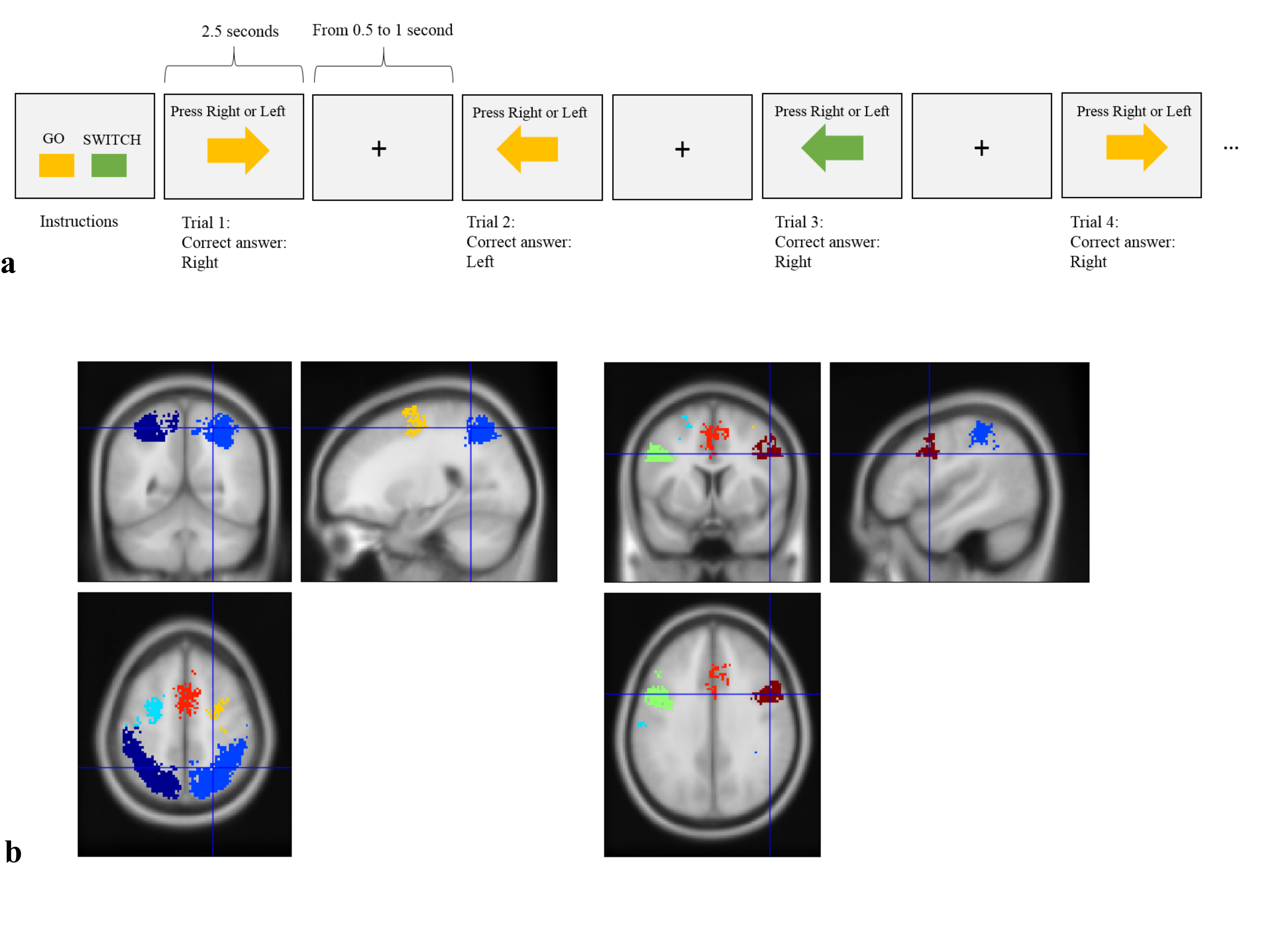
FMRI time series data were acquired from eleven healthy volunteers. The stimulus was a response inhibition task¹ as described in Fig.1a, and was repeated 5 times per sequence type using different acquisition parameters (Table.1). The order of the different protocols was counter-balanced across participants, while also ensuring that, for a given coverage and acceleration factor, the 3D and MB acquisitions were always consecutive.

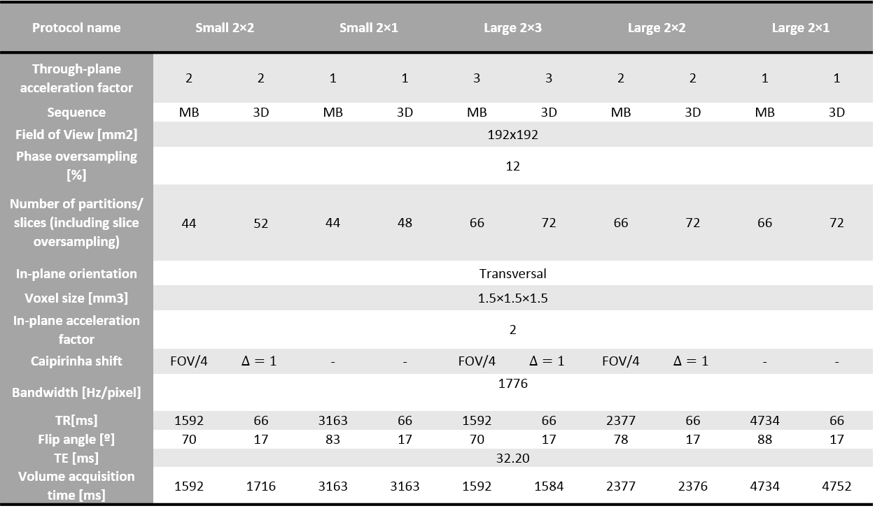
2D-MB-EPI scans were acquired with the gradient echo EPI sequence from the Center for Magnetic Resonance Research (R016,VE11C,https://www.cmrr.umn.edu/multiband/) while 3D-EPI-CAIPI scans were acquired with an in-house sequence². MB images were reconstructed with the GRAPPA-based algorithm provided with the sequence, while 3D images were reconstructed with a SENSE-based in-house algorithm implemented within Gadgetron³. Five protocols were tested for each sequence at 1.5mm isotropic resolution with a range of acceleration factors and coverage in the slice/slab-encoded direction. The EPI readout of the two approaches was matched. The flip angle was adjusted to the Ernst angle for each protocol assuming T1=1.5s. Respiration and cardiac traces were recorded.

All analyses were conducted in SPM12.3 (www.fil.ion.ucl.ac.uk/spm) using the General Linear Model (GLM) framework. Each time series was realigned to the first volume, corrected for distortion based on a B0 field map, co-registered to a T1-weighted image acquired in the same scanning session and normalised to the MNI space with the unified-segmentation algorithm⁴. Slice timing correction was applied to MB time-series.

Data were smoothed with different Gaussian kernel sizes (FWHM: 3,6 or 8mm) or not smoothed at all.

The GLM was composed of two conditions (SWITCH and GO), motion traces and physiological regressors⁵. Analysis without physiological regression was also performed. Data were high-pass filtered (>1/128Hz) and temporal correlations were modelled with the AR(1)+white noise model. A group analysis including all time-series of all participants was carried out to define seven regions of interest (ROI) based on activated clusters (p<0.05 FWE, extent threshold 100 voxels) (Fig.1.b). The average tSNR and the median of the highest 10% of t-scores for the contrast SWITCH>GO was computed in each ROI and for every protocol or processing pipeline. The tSNR was calculated as the estimated parameter of the constant term in the GLM divided by the standard deviation of the model residuals.

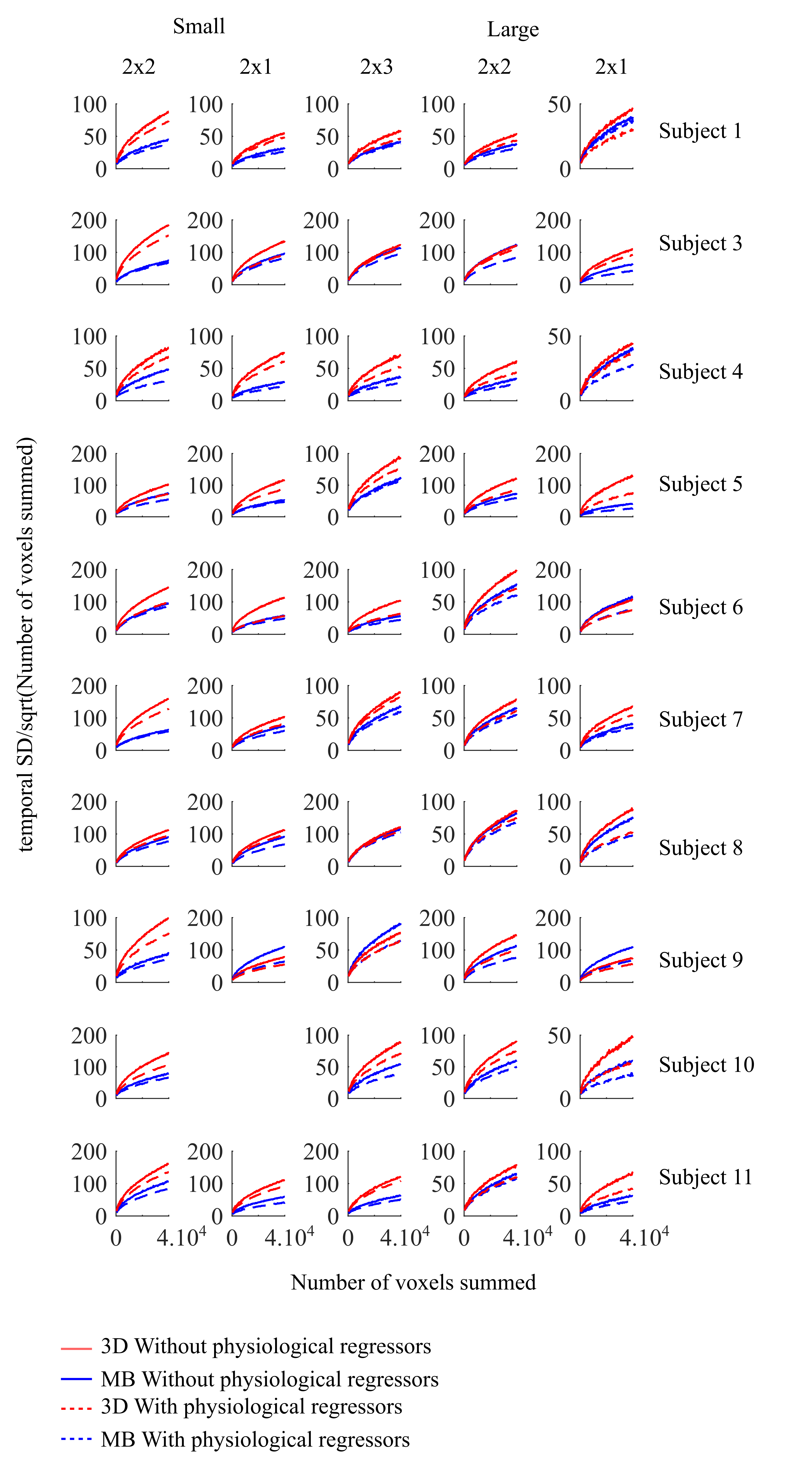
As shown in ⁶, spatial correlation in the noise limits the benefit of spatial smoothing in terms of tSNR. The hypothesis that 3D suffers from more spatial correlation and would therefore benefit less from smoothing was tested: Residuals of N randomly selected voxels $$$x_i$$$ within the grey matter mask (p(GM)>0.7) were added together and the temporal standard deviation of the summed voxels was computed and divided by $$$\sqrt N$$$ to account for the fact that the standard deviation of the sum of independent and normally distributed random variables increases with the square root of the number of summed variables. This step was repeated for $$$N\in[300:100:30000]$$$: $$f(N)= \frac{std(\sum_{i=1}^N x_i)}{\sqrt N}$$ The function f is expected to increase with N only in the presence of spatial correlation⁷.

Results

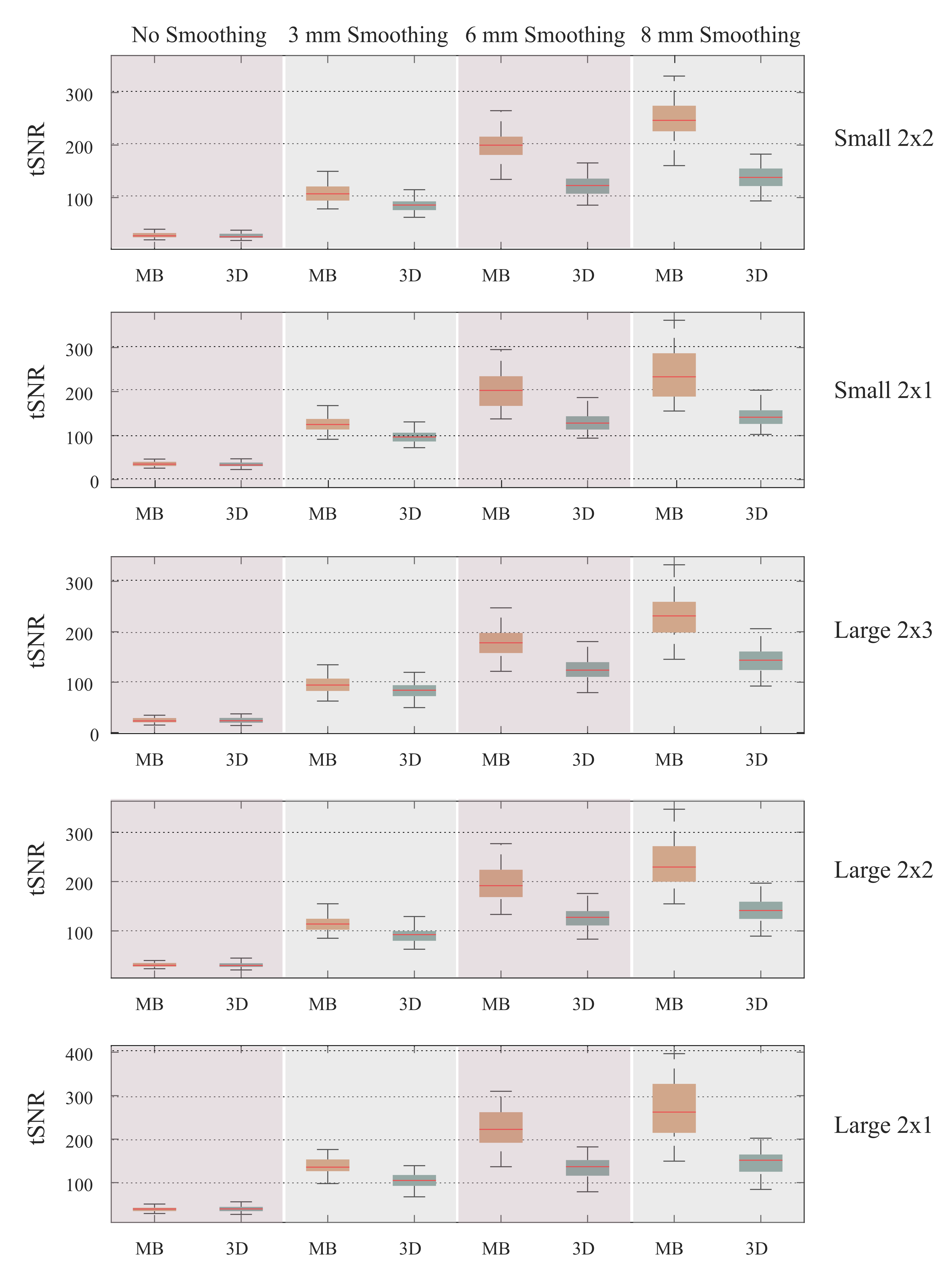
The average tSNR of 3D and MB was similar for a given protocol without smoothing (Fig.2). Increasing the smoothing kernel resulted in tSNR increases in both cases for every coverage/acceleration factor but to a greater extent for MB. The larger the smoothing kernel, the bigger the difference between the tSNR of 3D and MB.

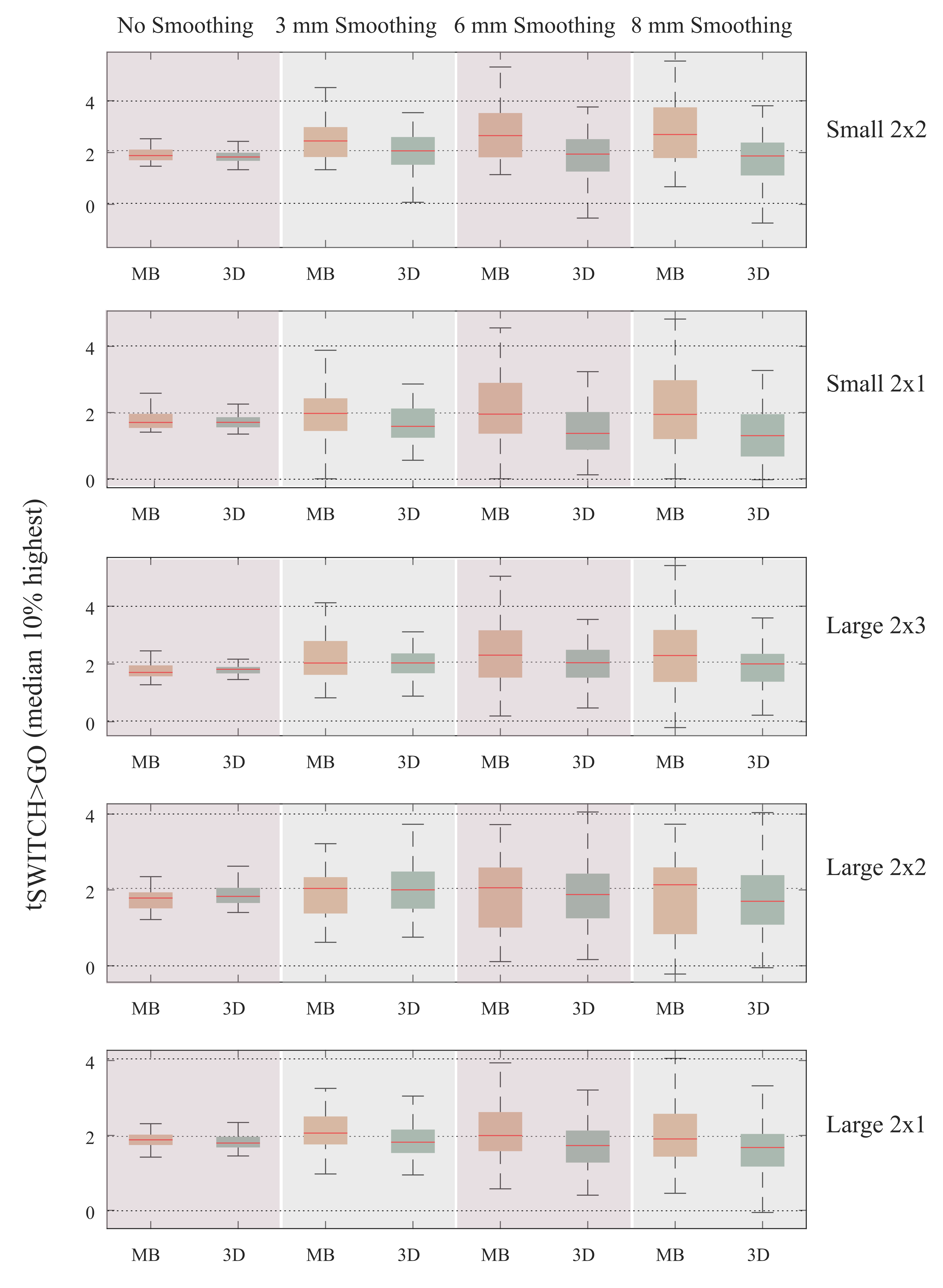
The median of the 10% highest t-score in the ROI also showed that MB benefited more from smoothing than 3D (Fig.3).

The measure f increased with increasing N for all protocols for both the 3D and MB acquisition schemes, indicating spatial correlation in the residuals (Fig.4). The 3D curves showed greater dependence on N than MB for 92% of the cases suggesting more spatial correlations with 3D, even when physiological noise correction was performed.

Conclusion

Acknowledgements

References

1. Kenner, N. M. et al. Inhibitory Motor Control in Response Stopping and Response Switching. J. Neurosci. 30, 8512–8518 (2010).

2. Narsude, M., Gallichan, D., van der Zwaag, W., Gruetter, R. & Marques, J. P. Three-dimensional echo planar imaging with controlled aliasing: A sequence for high temporal resolution functional MRI. Magn. Reson. Med. 75, 2350–2361 (2016).

3. Hansen, M. S. & Sørensen, T. S. Gadgetron: an open source framework for medical image reconstruction. Magn. Reson. Med. 69, 1768–1776 (2013).

4. Ashburner, J. & Friston, K. J. Unified segmentation. NeuroImage 26, 839–851 (2005).

5. Hutton, C. et al. The impact of physiological noise correction on fMRI at 7 T. NeuroImage 57, 101–112 (2011).

6. Triantafyllou, C., Hoge, R. D. & Wald, L. L. Effect of spatial smoothing on physiological noise in high-resolution fMRI. NeuroImage 32, 551–557 (2006).

7. Liu, C.-S. J. et al. Spatial and Temporal Characteristics of Physiological Noise in fMRI at 3T. Acad. Radiol. 13, 313–323 (2006).