3861
Classification of sleep stages from fMRI dynamic functional connectivity using deep learning1ISR-Lisboa/LARSyS and Department of Bioengineering, Instituto Superior Técnico - Universidade de Lisboa, Lisbon, Portugal, 2ISR-Lisboa/LARSyS and Department of Electrical Engineering, Instituto Superior Técnico - Universidade de Lisboa, Lisbon, Portugal, 3Department of Neurophysiology, Centro Hospitalar Psiquiátrico de Lisboa, Lisbon, Portugal
Synopsis
Sleep stage classifiers monitoring the wakefulness level of resting-state fMRI recordings have been proposed by several studies; however, the application of deep learning methods remains largely unexplored. We investigated the performance of Convolutional Neural Networks (CNNs) in the classification of sleep stages using fMRI-derived dynamic Functional Connectivity (dFC) features and simultaneous EEG-based labels. All tested architectures exhibited accuracies above 80%, with the best performance achieved using a shallow network. The learned filter weights were coherent with known stage-specific patterns of thalamo-cortical dFC. CNNs yielded comparable classification accuracy to Support Vector Machines (SVMs), without the need for exhaustive hyperparameter tuning.
Introduction
In the study of the brain’s functional connectivity (FC) based on resting-state fMRI, strong modulations of FC by wakefulness levels have been found1. This has motivated the development of sleep stage classifiers based on fMRI features, for the retrospective analysis of the data taking such modulations into account1-3. These classifiers were based on dynamic FC (dFC) features and resorted to conventional machine learning methods, namely Support Vector Machines (SVMs)1–3. Here, we aim to provide a proof-of-concept application of deep learning methods, particularly Convolutional Neural Networks (CNNs), to this problem.Methods
Data acquisition and pre-processing: An epileptic patient (male, 9 years old) underwent a simultaneous EEG-fMRI acquisition with a total duration of 30 minutes, during which alternation between wakefulness and sleep stages 1 and 2 was observed according to the EEG analysis by an expert neurophysiologist. BOLD-fMRI data were acquired using a 2D multi-slice GE-EPI sequence (TR/TE=2500/30ms, 40 axial slices, 3.5x3.5x3.0mm3). A T1-weighted structural image was also acquired (1mm isotropic). EEG data were recorded using an MR-compatible 32-channel system (Brain Products). EEG and fMRI data were pre-processed as described in a previous work4.
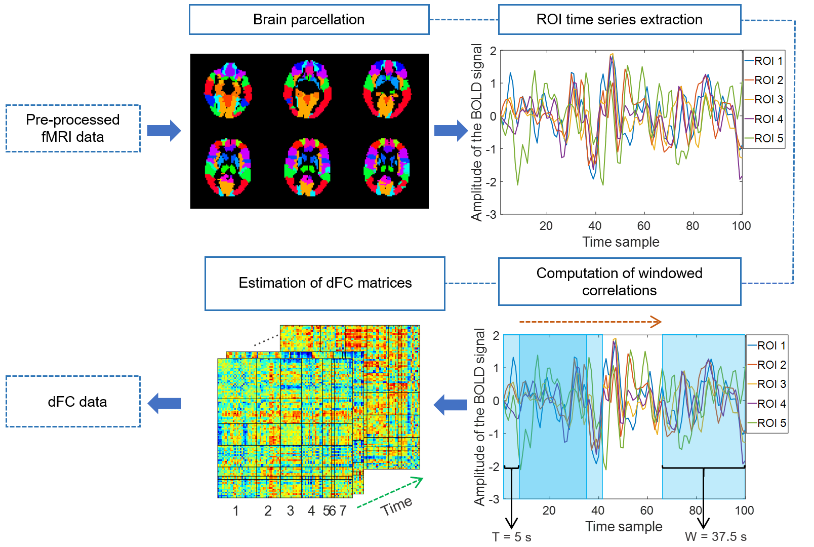
Estimation of dFC matrices: The estimation of dFC matrices (Fig.1) was performed using FSL-v5.0 (https://fsl.fmrib.ox.ac.uk/fsl/) and MATLAB-R2016b. Following brain parcellation into 90 ROIs defined by the AAL template5, representative BOLD time-series were obtained by within-ROI averaging and bandpass filtering (0.01-0.1Hz)6. dFC matrices were computed through a sliding-window Pearson correlation approach (window length= 37.5 s, step size=5 s), followed by the subtraction of the static FC matrix7.
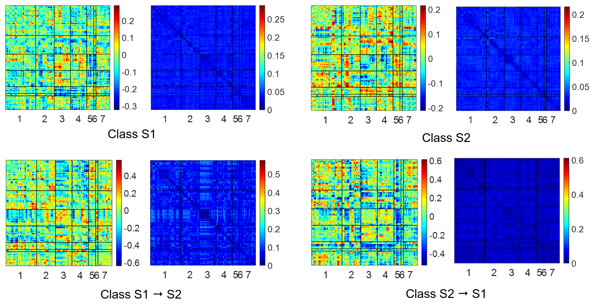
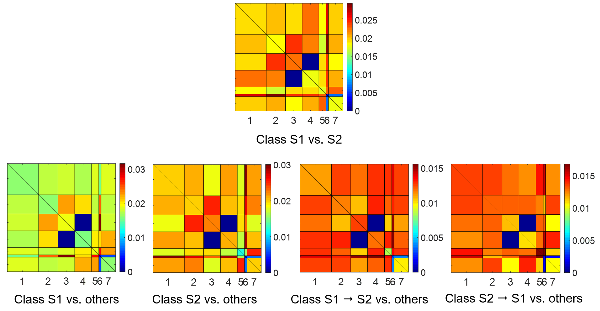
Image labeling: Every 30-s segment of the EEG dataset was assigned one sleep-stage label (S1 or S2) by a neurophysiologist8. Periods of time comprising more than one sleep stage were labeled as transition states (S1-S2 or S2-S1). This resulted in 4 classes with the following number of dFC matrices each: 99 for S1, 161 for S2, 21 for S1-S2 and for S2-S1. Within-class mean and standard error dFC matrices are presented in Fig.2.
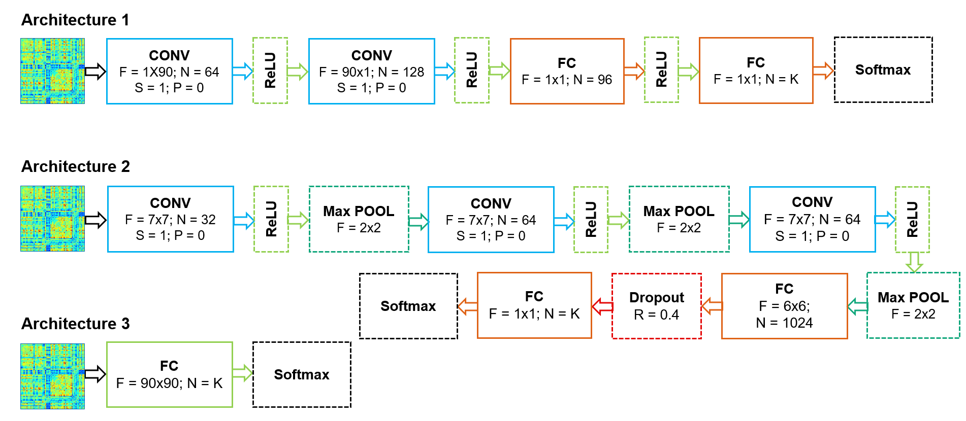
CNN implementation and training: CNN implementation was performed using MatConvNet (http://www.vlfeat.org/matconvnet/). The classification task was subdivided into a binary problem comprising classes S1 and S2 and a multi-class problem including the four classes. Three architectures (Fig.3) were evaluated: the filter design in Architecture 1 was inspired by the Connectome-CNN (CCNN) proposed by Meszlényi and colleagues9; Architecture 2 follows an AlexNet-like design10; and Architecture 3 comprises a single fully connected layer. The networks were trained using Stochastic Gradient Descent (SGD) with momentum and standard hyperparameter values.
Control tests: The following control tests were conducted using Architecture 3: in Control 1, average BOLD signal time-series in each ROI were used as features (1x90 vectors)11; in Control 2 and Control 3, phase randomization was applied to the ROI-averaged BOLD signal time-series11 and to the dFC matrices, respectively12.
Comparison with SVMs: A SVM with a radial basis function (RBF) kernel was applied3 using LIBSVM (https://www.csie.ntu.edu.tw/~cjlin/libsvm/) including a thorough hyperparameter optimization.
Results
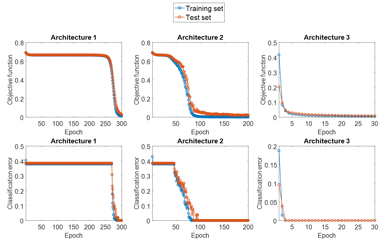
The evolution of the objective function and classification error over the epochs for the binary problem is presented in Fig.4 (a similar pattern was observed for the multi-class problem). The mean balanced accuracies obtained in the test data for the binary/multi-class problems were: 98.6/83.2%, 97.5/84.3% and 100.0/93.4% for Architectures 1, 2 and 3, respectively. The three control tests resulted in near chance-level balanced accuracies for both problems. Since Architecture 3 comprises a single fully connected layer, it was possible to directly analyze the weights attributed to each ROI’s FC values at the end of training (Fig.5). The application of SVMs to the binary/multi-class problems resulted in mean balanced accuracies of 100/92.9%.Conclusions
A good classification performance was obtained for the three CNN architectures, with balanced accuracies above 80%. The best results were achieved using Architecture 3, suggesting that no further feature extraction is required when using dFC features. The performance obtained for the binary problem was consistently superior to that of the multi-class problem, as expected considering the higher complexity of the discrimination task. A near chance-level accuracy was obtained when applying the three control tests, indicating that the original results were effectively driven by stage-specific dFC changes. In the binary problem, the highest difference of weights was verified for dFC involving the thalamus, which is coherent with the well-established involvement of thalamo-cortical FC during different sleep stages13,14. A comparison with SVMs revealed a similar performance on both problems but with a considerably superior computational cost. Further validation of the deep learning methods applied in this study is largely dependent on increased data availability.Acknowledgements
We acknowledge the Portuguese Science Foundation (FCT) for financial support through grants PTDC/EEIELC/3246/2012, UID/EEA/50009/2013 and PD/BD/105777/2014 and the P2020 Programme through grant LISBOA-01-0145-FEDER-029675.References
1. Tagliazucchi, E. & Laufs, H. Decoding Wakefulness Levels from Typical fMRI Resting-State Data Reveals Reliable Drifts between Wakefulness and Sleep. Neuron. 2014;82:695–708.
2. Altmann, A. et al. Validation of non-REM sleep stage decoding from resting state fMRI using linear support vector machines. Neuroimage. 2016;125: 544–555.
3. Tagliazucchi, E. et al. Automatic sleep staging using fMRI functional connectivity data. Neuroimage. 2012;63:63–72.
4. Abreu, R., Leal, A., Lopes da Silva, F. & Figueiredo, P. EEG synchronization measures predict epilepsy-related BOLD-fMRI fluctuations better than commonly used univariate metrics. Clin. Neurophysiol. 2018; 129:618–635.
5. Tzourio-Mazoyer, N. et al. Automated anatomical labeling of activations in SPM using a macroscopic anatomical parcellation of the MNI MRI single-subject brain. Neuroimage. 2002;15:273-289.
6. Gonzalez-Castillo, J. & Bandettini, P. A. Task-based dynamic functional connectivity: Recent findings and open questions. NeuroImage. 2017;180:526-533.
7. Leonardi, N., Shirer, W. R., Greicius, M. D. & Van De Ville, D. Disentangling dynamic networks: Separated and joint expressions of functional connectivity patterns in time. Hum. Brain Mapp. 2014;35:5984–5995.
8. Rechtschaffen, A. A manual for standardized terminology, techniques and scoring system for sleep stages in human subjects. Brain Research Institute. US Department of Health, Education, and Welfare, 1968.
9. Meszlényi, R. J., Buza, K. & Vidnyánszky, Z. Resting State fMRI Functional Connectivity-Based Classification Using a Convolutional Neural Network Architecture. Front. Neuroinform. 2017;11:1–12.
10. Krizhevsky, A., Sutskever, I. & Hinton, G. E. ImageNet Classification with Deep Convolutional Neural Networks. Adv. Neural Inf. Process. Syst. 2012;1-9.
11. Gonzalez-Castillo, J. et al. Tracking ongoing cognition in individuals using brief, whole-brain functional connectivity patterns. Proc. Natl. Acad. Sci. 2015;112(28):8762–8767.
12. Allen, E. A. et al. Tracking whole-brain connectivity dynamics in the resting state. Cereb. Cortex. 2014;24(3):663–676.
13. Picchioni, D., Duyn, J. H. & Horovitz, S. G. Sleep and the functional connectome. Neuroimage. 2013;80:387–396.
14. Tagliazucchi, E. & van Someren, E. J. W. The large-scale functional connectivity correlates of consciousness and arousal during the healthy and pathological human sleep cycle. Neuroimage. 2017;160:55–72.
Figures