3824
k-space MR Thermometry Using k-space Energy Spectrum Analysis1Biomedical Instrument Institute, School of Biomedical Engineering, Shanghai Jiao Tong University, Shanghai, China, 2Department of Radiology, Brigham and Women's Hospital, Boston, MA, United States, 3Med-X Research Institute, School of Biomedical Engineering, Shanghai Jiao Tong University, Shanghai, China, 4Department of Physics, Soochow University, Taipei, Taiwan
Synopsis
The goal of this work was to perform MR thermometry in the k-space domain, as opposed to the image domain, on the premise that a k-space approach might be better suited at capturing spatial trends. The method relies on the fact that spatial gradients in temperature cause k-space shifts in signals for heated materials. Traditional proton resonance frequency (PRF) thermometry was also performed, for validation purposes.
Introduction
MR thermometry plays an important role in MR-guided focused ultrasound surgery (MRgFUS). The proton resonant frequency (PRF) effect allows temperature changes to be detected and temperature dose to be calculated. The PRF effect causes temperature-dependent phase shifts, which are typically detected in the object domain. The present work explores complementary detection of PRF effects in the k-space domain, where spatial variations in temperature might be more readily detected and quantified. In the k-space domain, spatial gradients in temperature take the form of k-space shifts, i.e., spatial temperature gradients effectively displace the signals of heated materials in k-space1,2.Methods
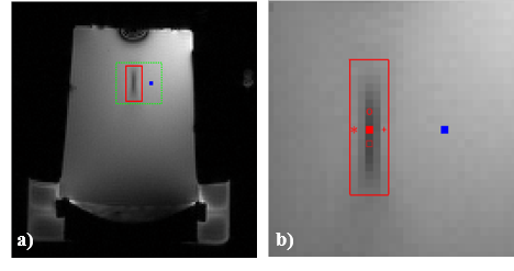
Focused ultrasound (FUS) heating was performed in a gel phantom, see Fig. 1. Imaging was performed on a GE Signa 3.0T system using an RF-spoiled gradient echo sequence (TR=25.0 ms, TE=16.5 ms, FOV=19.2×19.2 cm2, matrix size=128×128, bandwidth=±10.0 kHz). For FUS heating, a circular single-element 1.5 MHz transducer with 50-mm radius was employed. This transducer was curved in the depth dimension to create a natural focus point, and this curvature was characterized by a 100-mm radius. During FUS experiments, the transducer delivered 78 W of acoustic power over a 20 s period. The red rectangle in Fig. 1a marks the focal area, with maximum heating, while the small blue square indicates a reference non-heated location.
The resulting data were analyzed in k-space using an algorithm related to the ‘k-space energy spectrum analysis’ (KESA) method2. The purpose of the processing was to detect k-space shifts associated with spatial gradients in temperature. As in KESA, increasingly-large swaths of the kx axis were replaced with zeros while monitoring the effect on the signal intensity at all pixels. The signal intensity as a function of the zero-filling extent can be plotted for any given pixel; for signal shifted in k-space away from k-space center, signal will drop most precipitously when these k-space locations get replaced with zeros.
The temperature variation associated with k-space shift is computed based on the following equation: Δ(dT/dx)=Δk/(γ·α·B0·TE·N), where Δk is the k-space shift in pixel number, Δ(dT/dx) is the temporal change of temperature gradient in space, N is the matrix size in frequency encoding direction, γ is the gyromagnetic ratio for hydrogen (42.58 MHz/T), α is the PRF change coefficient (−0.01 ppm/°C), B0 is the main field strength.
Results
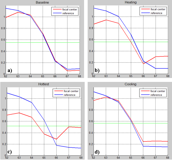
As can be seen in Fig. 2, the signal in a heated pixel gets k-space shifted with respect to a reference non-heated pixel. Blue and red curves correspond to the blue and red pixels in Fig. 1b, respectively. Figure 2a shows the reference and heated pixel with the main bulk of their signal at essentially the same location in k-space, but an increasingly-large shift develops with heating (Fig. 2b, then 2c) and comes back to nearly zero after cooling (Fig. 2d). This method can be employed to find temperature gradients at all spatial locations and all time points, then a k-shift map can obtain (see Fig. 3a) and a temperature elevation map can be calculating through spatial integration (see Fig. 4).
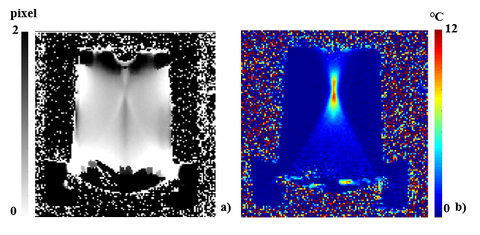
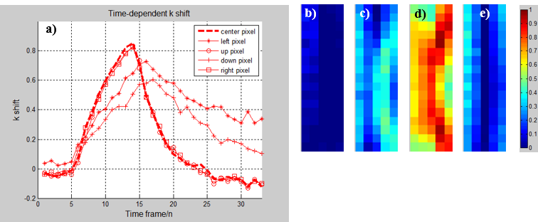
The heated k-shift map and corresponding temperature map are shown in Fig. 3a and Fig. 3b respectively for the heated phantom in Fig. 1. These maps show the k-shift pixels and temperature change distributions for the time frame with maximum heating. Time-dependent k-shift plots are shown in Fig. 4a for the five locations indicated with red markers in Fig. 1b. Through spatial integration along x, a temperature elevation map was obtained in Fig. 4b from the measured gradients, and compared in Fig. 4c to a map directly obtained in the spatial domain.
Discussion and Conclusion
Temperature-induced frequency shifts were detected here in k-space rather than in the object domain, as would normally be done in PRF imaging. Because k-space detection may be more sensitive to spatial gradients in temperature rather than the temperature itself, we believe the two approaches may have complementary value toward generating accurate temperature maps, especially in the presence of noise.Acknowledgements
Thanks to the support from 2015 and 2017 Key Project of Shanghai Science and Technology Commission (No. 15441900700, 17441906400), National Key Research and Development Program of Ministry of Science and Technology (No. 2017YFC0108900) and National Natural Science Foundation of China (No. 81727806, 11774231).References
[1] C.-S. Mei, R. Chu, W. S. Hoge, L. P. Panych, and B. Madore, “Accurate field mapping in the presence of B0 inhomogeneities, applied to MR thermometry,” Magnetic Resonance in Medicine, vol. 73, no. 6, pp. 2142–2151, Jun. 2015.
[2] N. Chen, K. Oshio, and L. P. Panych, “Application of k-space energy spectrum analysis to susceptibility field mapping and distortion correction in gradient-echo EPI,” NeuroImage, vol. 31, no. 2, pp. 609–622, Jun. 2006.
Figures