3767
Revisiting mental chronometry with isotropic resolution and full brain coverage.1Donders Institute for Brain, Cognition and Behaviour, Radboud University, Nijmegen, Netherlands, 2Erwin L. Hahn Institute for Magnetic Resonance Imaging, Essen, Germany
Synopsis
In this project, we are using a multiband echo-shifted EPI sequence for TR less than 160 ms combined with a novel analysis approach to measure interregional BOLD onset times from a visual-motor association task with full brain coverage and isotropic resolution.
Introduction
Functional MRI (fMRI) uses the blood oxygenation level dependent (BOLD) contrast to study the hemodynamic responses associated with neuronal activity1, however, conventional fMRI sequences cannot be used to measure intraregional BOLD onset latencies because of their slow sampling rate. Ultrafast fMRI (TR < 200ms), overcomes these problems and can be used to extract the relative timing information from different areas of the brain, and thus enables probing the order in which these regions may be engaged to perform a task, i.e., enables "mental chronometry”. This approach has been used previously, albeit with limited brain coverage, to find (0~100ms) differences in BOLD onset times across different brain areas 2,3. In the study conducted by Menon et al., BOLD response onsets in the motor planning areas were shown to correlate with behavioral reaction times4,5,6. In the current contribution, we expand on Menon et al.’s experiment using a multiband echo-shifted EPI7 sequence combined with a novel analysis approach to measure interregional BOLD onset times from a visual-motor association task with full brain coverage and isotropic resolution.Methodology
Data Acquisition
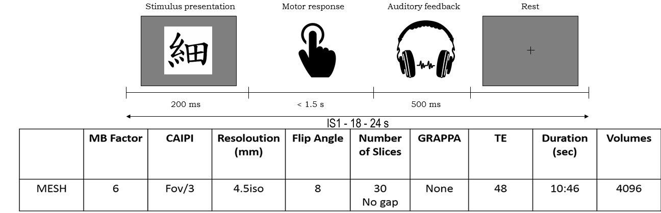
Data were collected from five (26±3.18) right-handed subjects on a 3T MRI scanner (Prisma, Siemens Healthcare, Erlangen, Germany) equipped with a 32-channel head coil. FMRI data were acquired with a multiband echo-shifted (MESH) EPI sequence using imaging parameters given in Table 1. Single slice reference images were collected prior to image acquisition to separate MB slices using SplitSlice-GRAPPA, also known as LeakBlock8,9 The visual motor association task used for the experiment is shown and described in Figure 1A.
Data Preprocessing
fMRI data were preprocessed using FMRIPREP version 1.1.33 10, a Nipype4 based tool11. All fMRI data were motion corrected, distortion correction with ANTs antsRegistration, boundary-based rigid registration using FSL FLIRT. The preprocessed data were high pass filtered and cleaned for physiological noise by running Spatial ICA from FSL, choosing the components related to the physiological noise and, removing them using FSL- REGFILT. In the preprocessing, and analysis, no smoothing was applied to minimize partial volume effects. Data were bandpass filtered between 10-50 Hz to remove cardiac fluctuation leading to smoothed time-courses.
Data Analysis
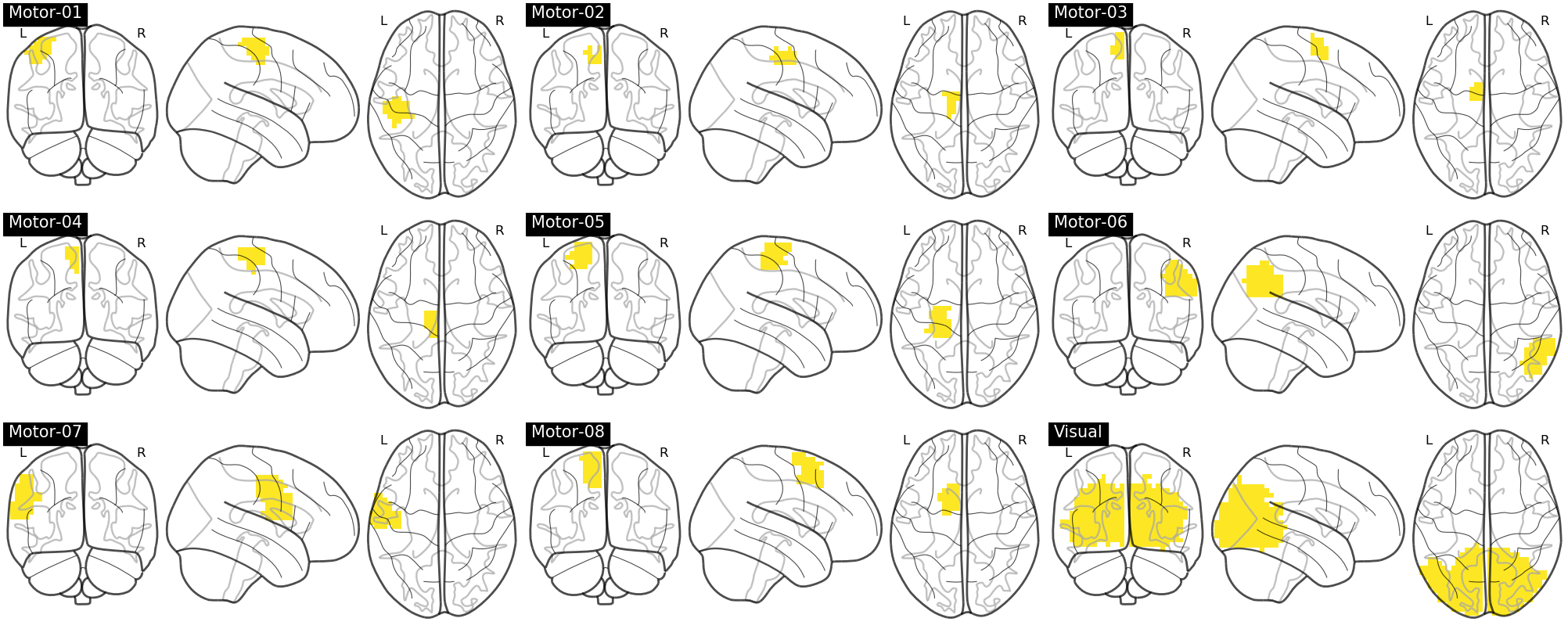
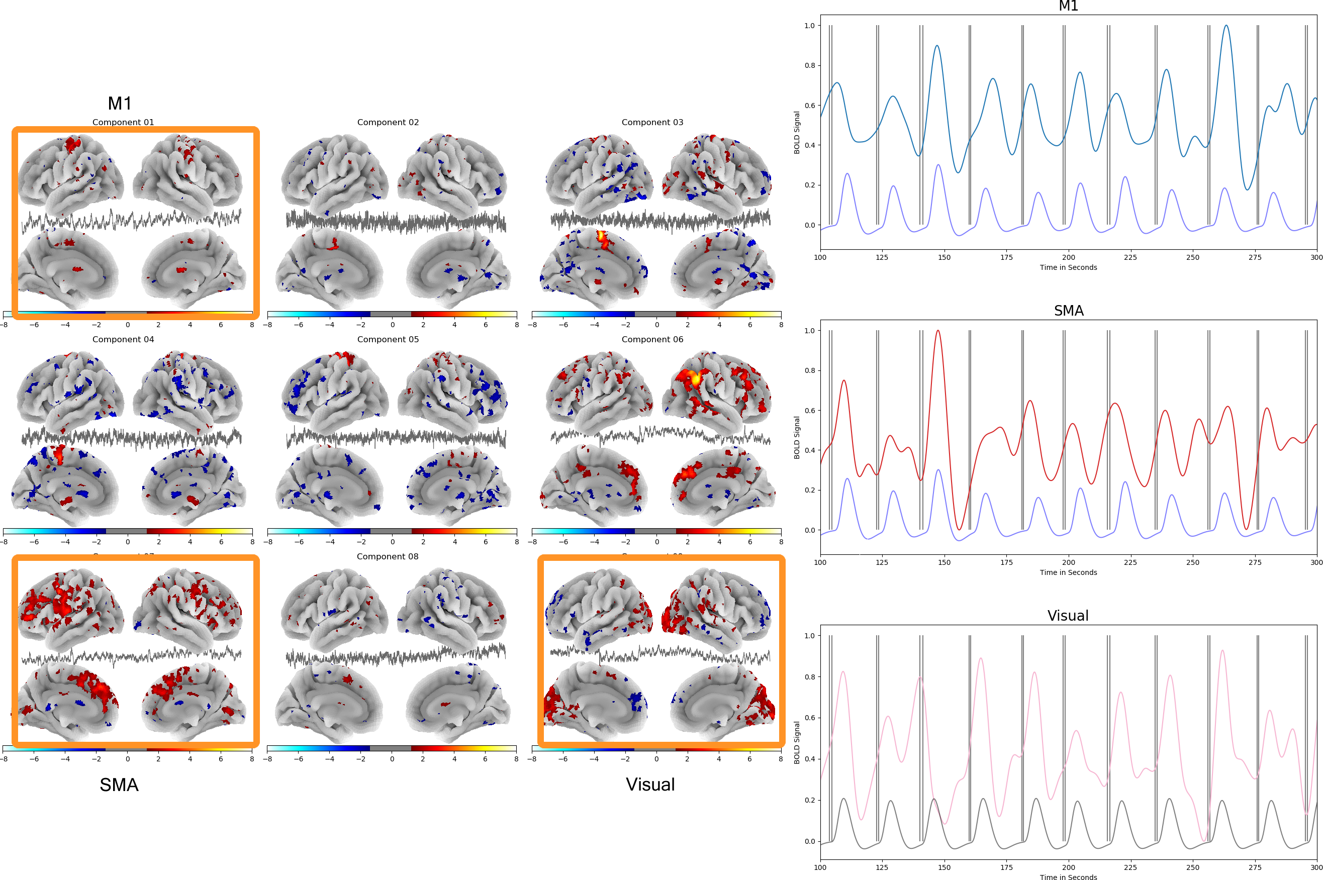
To separate functional regions, we used dual regression for which we created our own template of nine selected components from the Multiresolution Intrinsic Segmentation Template (MIST) atlas12, (Figure 2). In this template, we have eight motor components and one visual component. Using this template dual regression gave us a participant-specific time series for each component. Next, these time series were entered in a multivariate temporal regression against the task regressors (including stimulus and reaction time regressors), resulting in participant-specific parameter estimate (PE) and Z-statistical maps. Among the activated regions, we selected two motor and one visual component (corresponding roughly to M1, SMA, and early visual areas) with high correlations with the reaction time and stimulus regressors respectively. These are shown by the highlighted surface map in Figure 3A. The correlation is depicted in Figures 3B, 3C and 3D. For each region all 34 trials were averaged and the time to peak calculated by taking t=0 as the time at which the visual stimulus is presented. Linear regression was used to fit a line to the 20-70 % of the peak height and the intercept of this line was taken as the onset of hemodynamic response. The onset difference between any two regions is defined as the difference between the two onset points.
Results
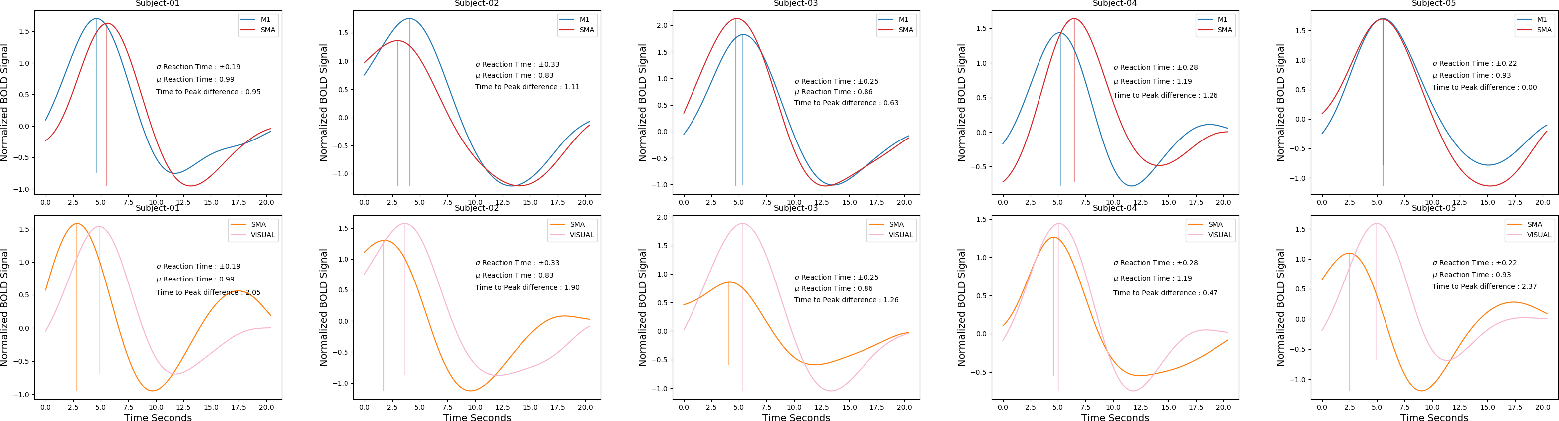
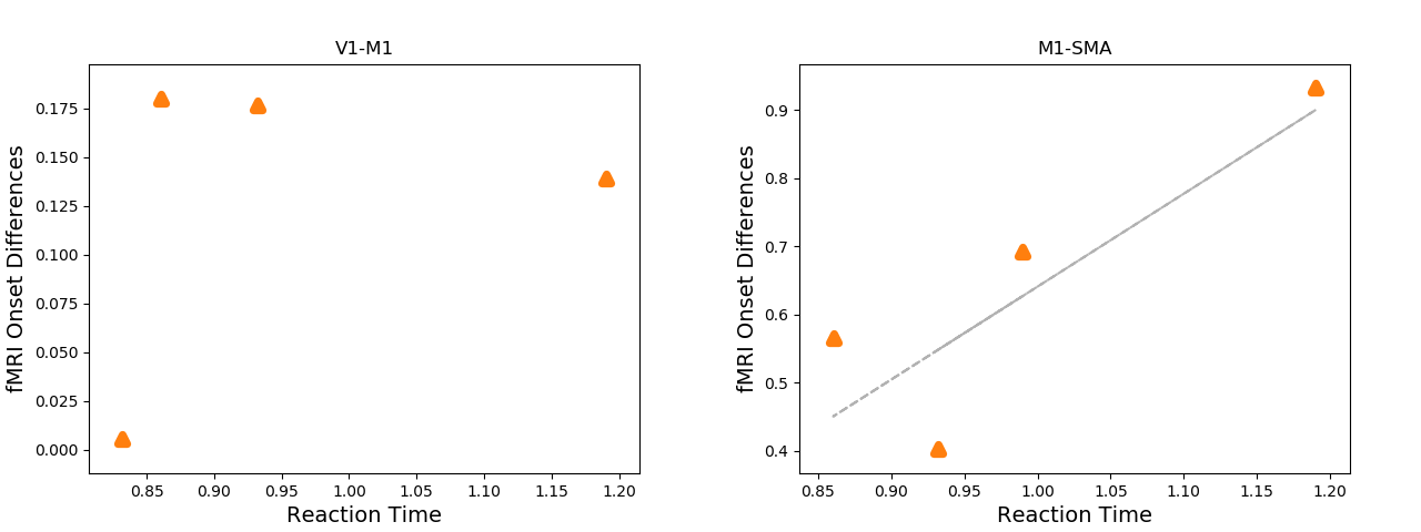
Figure 4A examines time to peak differences between M1/SMA (A) and M1/visual (B). We observe that there is time to peak differences between the motor areas, but not between M1 and visual, in accordance with1. In Figure 5, the onset differences between the hemodynamic responses from visual to M1 (5A) and SMA-M1 (5B) are plotted against the measured reaction times.Discussion and Conclusion
We have shown that it is possible to measure timing differences between different areas of the brain with an ultrafast fMRI sequence with full brain coverage and isotropic resolution. We could replicate Menon’s 1998 findings and show that BOLD onset times correlate with reaction times. This will help better understand the temporal hierarchy of the different cognitive processes in the brain depending on the task, and opens the door to examining the duration of mental processes in the brain with fMRI.Acknowledgements
No acknowledgement found.References
1. Ogawa S, Menon RS, Tank DW, Kim SG, Merkle H, Ellermann JM, et al. Functional brain mapping by blood oxygenation level-dependent contrast magnetic resonance imaging. A comparison of signal characteristics with a biophysical model. Biophys J. 1993 Mar;64(3):803–12. 2. Menon RS. Mental chronometry. Neuroimage. 2012 Aug 15;62(2):1068–71. 3. Menon RS, Kim S-G. Spatial and temporal limits in cognitive neuroimaging with fMRI. Trends Cogn Sci. 1999 Jun 1;3(6):207–16. 4. Chang C, Thomason ME, Glover GH. Mapping and correction of vascular hemodynamic latency in the BOLD signal. 2008; 5.Menon RS, Luknowsky DC, Gati JS. Mental chronometry using latency-resolved functional MRI. Proc Natl Acad Sci. 1998;95(18):10902–7. 6. Richter W, Ugurbil K, Georgopoulos A, Kim SG. Time-resolved fMRI of mental rotation. Neuroreport. 1997;8(17):3697–702. 7. Boyacioğlu R, Schulz J, Norris DG. Multiband echo-shifted echo planar imaging. Magn Reson Med. 2017;77(5):1981–6. 8. Setsompop K, Gagoski BA, Polimeni JR, Witzel T, Wedeen VJ, Wald LL. Blipped-controlled aliasing in parallel imaging for simultaneous multislice echo planar imaging with reduced g-factor penalty. Magn Reson Med. 2012 May 1;67(5):1210–24. 9. Cauley SF, Polimeni JR, Bhat H, Wang D, Wald LL, Setsompop K. Inter-slice Leakage Artifact Reduction Technique for Simultaneous Multi-Slice Acquisitions. 10. Esteban O, Markiewicz CJ, Blair RW, Moodie CA, Ilkay Isik A, Erramuzpe A, et al. ARTICLE PRE-PRINT FMRIPrep: a robust preprocessing pipeline for functional MRI. 11. Gorgolewski K, Burns CD, Madison C, Clark D, Halchenko YO, Waskom ML, et al. Nipype: A Flexible, Lightweight and Extensible Neuroimaging Data Processing Framework in Python. Front Neuroinform. 2011;5(August). 12. Urchs S, Armoza J, Benhajali Y, St-Aubin J, Orban P, Bellec P. MIST: A multi-resolution parcellation of functional brain networks. MNI Open Res. 2017;1(0):3.Figures