3748
BOLD Representation of Canonical EEG Microstates1Laureate Institute for Brain Research, Tulsa, OK, United States, 2Electrical and Computer Engineering, University of Oklahoma, Norman, OK, United States, 3Japan Society for the Promotion of Science, Tokyo, Japan, 4Stephenson School of Biomedical Engineering, University of Oklahoma, Norman, OK, United States
Synopsis
We extracted the topographical similarity of EEG signals with four canonical EEG microstate (EEG-ms, A through D) templates from 47 healthy subjects. Then, a general linear model (GLM) examined topographical similarities using time courses convolved with hemodynamic response function (HRF) as regressors of interest for individual subjects. A one-sample t-test was applied
Purpose
In awake and resting brains, spontaneous and large-scale hemodynamic fluctuations in brain activity are spatially organized and temporally correlated into specific functional networks, as measured by blood-oxygenation-level-dependent functional MRI (BOLD fMRI). On the other hand, the spatio-temporal analysis of resting state EEG signal activity has revealed the presence of a number of quasi-stable topographic representations of EEG potentials, called EEG microstates (EEG-ms)1,2,3. The four identified spatially independent EEG-ms are coined canonical microstates A through D. EEG-ms provide an opportunity to study the relationship between EEG and fMRI signals4,5,6. In this study, we adopted the spatial similarity of each EEG sample to four canonical EEG-ms as regressors of interest in GLM of whole brain fMRI analysis. Identifying BOLD representations of EEG microstates provides some insight into the relationship between EEG and fMRI signals and may provide a better understanding of resting state activity.Methods
Participants: 47 healthy subjects (24 females, age 18-54) were selected from the Tulsa 1000 dataset7 for the analysis. Simultaneous EEG-fMRI resting state data obtained for each participant and was used for analysis (fMRI: TR/TE=2000/27ms, 8min; EEG: 32 channels). AFNI was used for fMRI analysis (https://afni.nimh.nih.gov/) with these preprocessing steps: the first three volumes were omitted, despike, RETROICOR8 was used for respiration- and cardiac-induced noise correction, slice-timing and motion corrections, spatial smoothing with FWHM=6mm kernel, and scaling signal to percent change. We followed the EEG preprocessing pipeline9 to remove imaging and BCG artifacts. Additionally, residual BCG, ocular and muscle artifacts were removed using ICA. The EEG-ms analysis was conducted by calculating the peaks of the global field power (GFP) after reference-averaging3. Next, the atomize and agglomerate hierarchical clustering AAHC algorithm was used to segment the EEG points while fixing the number of desired microstates at four (k=4). Using the peaks of GFP for each subject, we selected the corresponding EEG points and submitted them to AAHC. After that, we computed the group mean of EEG-ms by first sorting individual EEG-ms and then finding common topographies across all subjects. Finally, individual subjects were ordered based on the group mean. We calculated the spatial similarity between each EEG time point and group mean templates. The time series was convolved with the Hemodynamic Response Function (HRF) from AFNI and down-sampled to the temporal resolution of fMRI. GLM used the four regressors from each subject along with six motion parameters, their temporal derivatives, three principal components of ventricle signal and local white matter average signal (ANATICOR10). One-sample t-tests were applied to the regression coefficients of the GLM analysis at the group level. Estimating a cluster correction with the ACF11 option revealed that 196 voxels were needed to control false positives with p=0.005 and α=0.05.Results
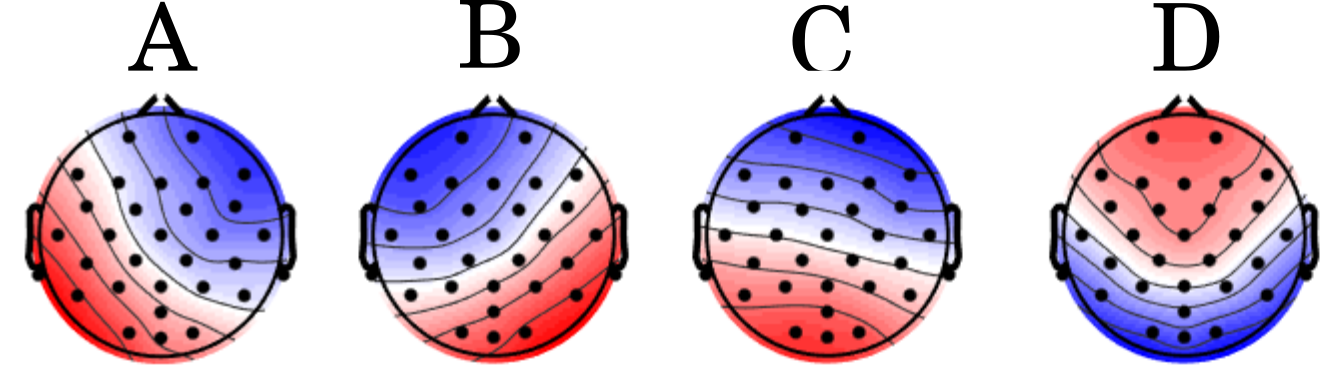
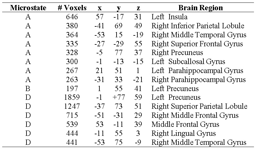
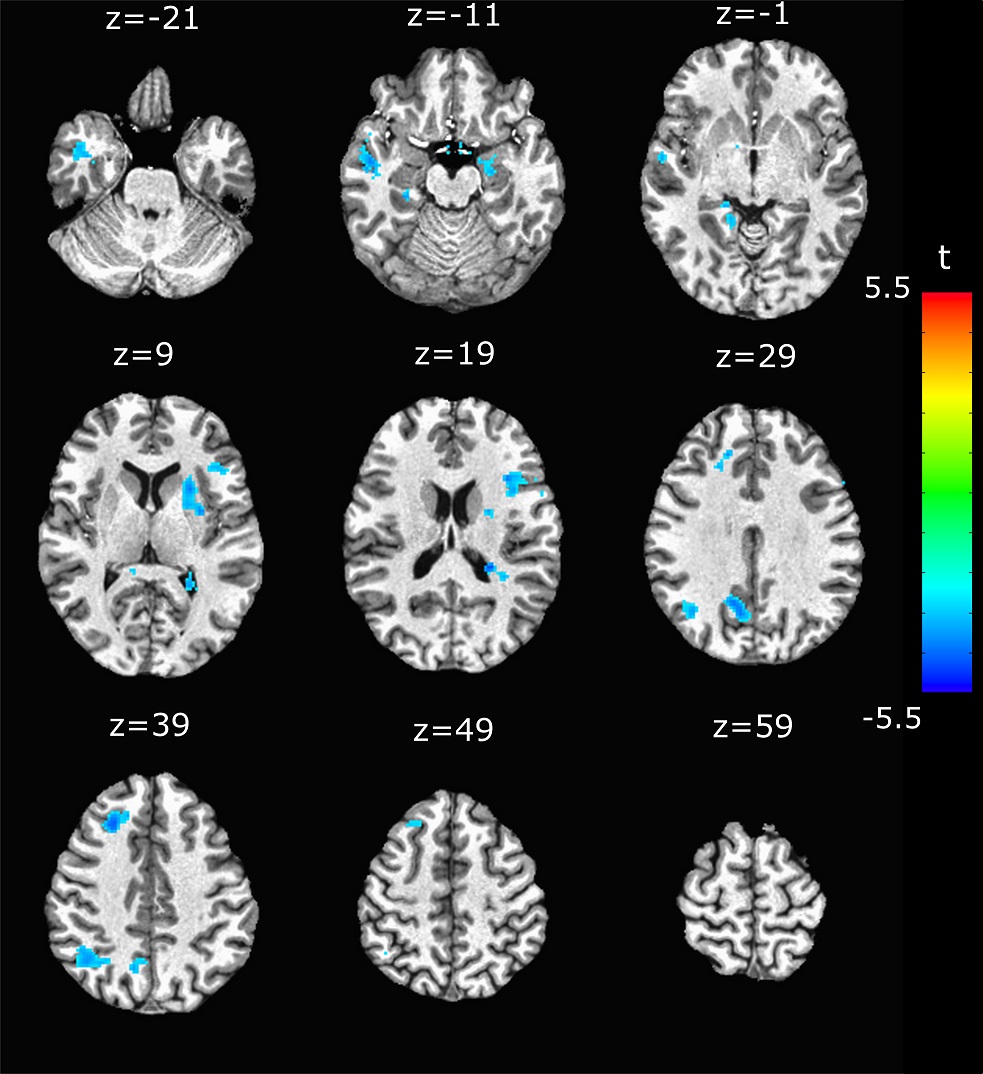
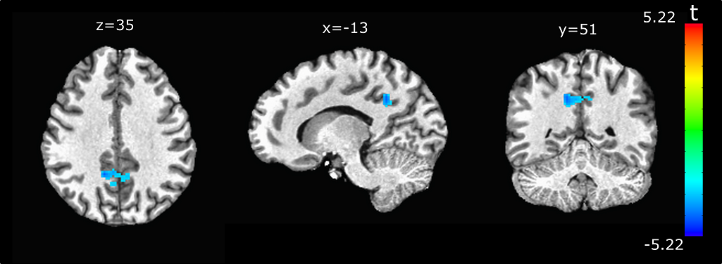
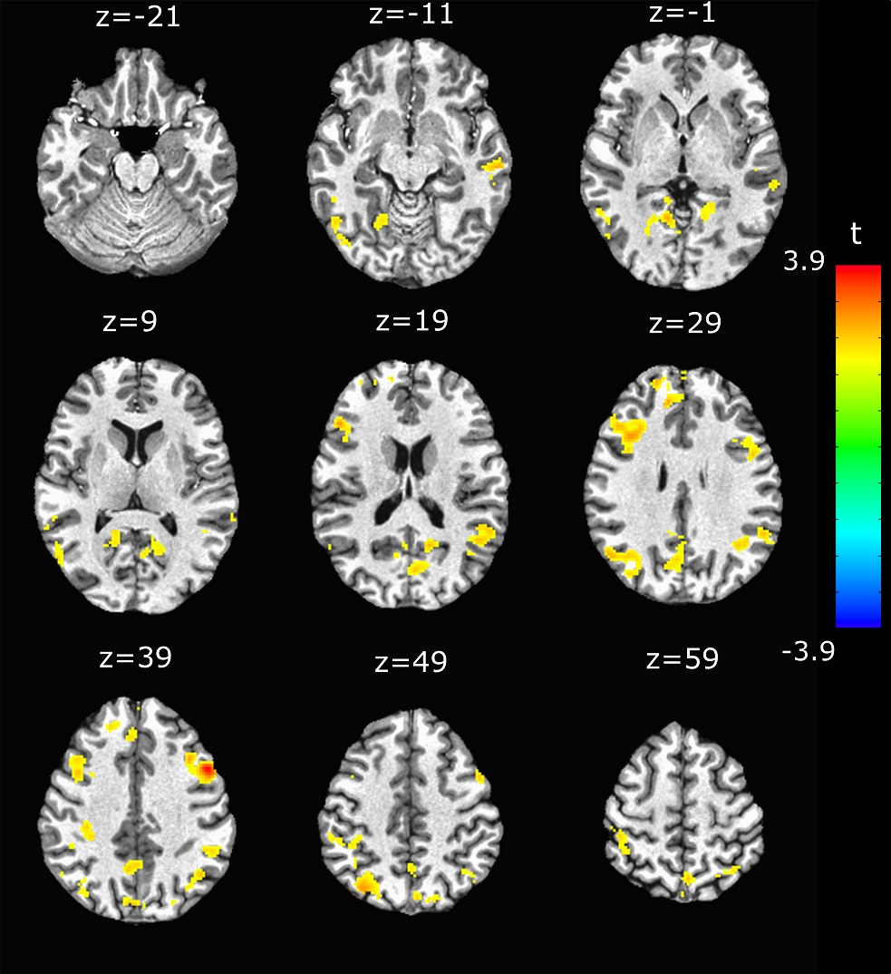
Figure 1 shows the EEG-ms templates. Figure 2 details the brain regions associated with each microstate. Figures 3, 4, 5 show the significant clusters extracted from the clustering analysis.Discussion
We have identified the presence of the four canonical EEG-ms in our EEG datasets and provided a replication of the previous reports4,6. The spatial similarities of EEG topography, used as regressors for the GLM analysis, revealed the BOLD representation of EEG-ms. Several brain regions (Figure 2) were associated with microstates A, B, and D. No association was found for microstate C. Some of the brain regions are similar to those obtained by other works4,6. However, it is difficult to make direct comparisons due to differences in the datasets. For example, we used eyes open with a significantly larger number of subjects as opposed to eyes closed, which was used in the previous works4,6. Examining other types of regressors, like average duration and occurrence, may provide a better understanding of the meaning of scale-free time association between EEG-ms and BOLD.Acknowledgements
This work has been supported by the Laureate Institute for Brain Research, The William K. Warren Foundation, and by National Institute of General Medical Sciences, National Institutes of Health Award 1P20GM121312. Tulsa 1000 investigators: Robin L Aupperle1,5, Sahib S. Khals1,5, Justin S. Feinstein1,5, Jonathan Savitz1,5, Yoon-Hee Cha1,5, Rayus Kuplicki1, Teresa A Victor1
1Laureate Institute for Brain Research
5Oxley College of Health Sciences, University of Tulsa, Tulsa, Oklahoma, USA
References
1. Lehmann, Dr, H Ozaki, and I Pal. "Eeg Alpha Map Series: Brain Micro-States by Space-Oriented Adaptive Segmentation." Electroencephalography and clinical neurophysiology 67.3 (1987): 271-88.
2. Khanna, Arjun, et al. "Microstates in Resting-State Eeg: Current Status and Future Directions." Neuroscience & Biobehavioral Reviews 49 (2015): 105-13.
3. Michel, Christoph M, and Thomas Koenig. "Eeg Microstates as a Tool for Studying the Temporal Dynamics of Whole-Brain Neuronal Networks: A Review." NeuroImage (2017).
4. Musso, Francesco, et al. "Spontaneous Brain Activity and Eeg Microstates. A Novel Eeg/Fmri Analysis Approach to Explore Resting-State Networks." Neuroimage 52.4 (2010): 1149-61.
5. Yuan, Han, et al. "Spatiotemporal Dynamics of the Brain at Rest—Exploring Eeg Microstates as Electrophysiological Signatures of Bold Resting State Networks." Neuroimage 60.4 (2012): 2062-72.
6. Britz, Juliane, Dimitri Van De Ville, and Christoph M Michel. "Bold Correlates of Eeg Topography Reveal Rapid Resting-State Network Dynamics." Neuroimage 52.4 (2010): 1162-70.
7. Victor, Teresa A, et al. "Tulsa 1000: A Naturalistic Study Protocol for Multilevel Assessment and Outcome Prediction in a Large Psychiatric Sample." BMJ open 8.1 (2018): e016620.
8. Glover, Gary H, Tie‐Qiang Li, and David Ress. "Image‐Based Method for Retrospective Correction of Physiological Motion Effects in Fmri: Retroicor." Magnetic Resonance in Medicine: An Official Journal of the International Society for Magnetic Resonance in Medicine 44.1 (2000): 162-67.
9. Mayeli, Ahmad, et al. "Real-Time Eeg Artifact Correction During Fmri Using Ica." Journal of neuroscience methods 274 (2016): 27-37.
10. Jo, Hang Joon, et al. "Mapping Sources of Correlation in Resting State Fmri, with Artifact Detection and Removal." Neuroimage 52.2 (2010): 571-82.
11. Cox, Robert W, et al. "Fmri Clustering in Afni: False-Positive Rates Redux." Brain connectivity 7.3 (2017): 152-71.
Figures