3746
Classification of BOLD-fMRI dynamic functional connectivity states based on simultaneous EEG microstates1ISR-Lisboa/LARSyS and Department of Bioengineering, Instituto Superior Ténico, Universidade de Lisboa, Lisboa, Portugal, 2Coimbra Institute for Biomedical Imaging and Translational Research (CIBIT) and CNC.IBILI, University of Coimbra, Coimbra, Portugal, 3Department of Neurophysiology, Centro Hospitalar Psiquiátrico de Lisboa, Lisboa, Portugal
Synopsis
Dynamic functional connectivity (dFC) states have been identified in BOLD-fMRI data, but their electrophysiological underpinnings remain a matter of debate. The simultaneous acquisition of the EEG has previously allowed the identification of EEG signatures of dFC states. Here, we further investigated whether EEG microstates can be used to classify dFC states. We found that highly accurate classification could be achieved based on the three EEG microstates with the highest global explained variance, in simultaneous EEG-fMRI data acquired from eight epileptic patients. These results further support the electrophysiological underpinnings of fMRI dFC states, highlighting their relationship with EEG-derived microstates.
Introduction
The identification of dynamic functional connectivity (dFC) states from BOLD-fMRI data has raised great interest regarding our understanding of functional brain networks, particularly given their potential as disease biomarkers1. However, the electrophysiological underpinnings of such dFC states remain a matter of debate. A previous study identified EEG spectral signatures of dFC states measured during eyes opening and closing2. We have recently identified EEG signatures of dFC epileptic states based on both spectral features and microstates3. Here, we aim to further investigate whether EEG microstates can be used to classify fMRI dFC states in general. For this purpose, we estimate EEG microstates using two different approaches, and feed them into a random forests classifier to discriminate fMRI dFC states, in simultaneous EEG-fMRI data from eight epileptic patients.Methods
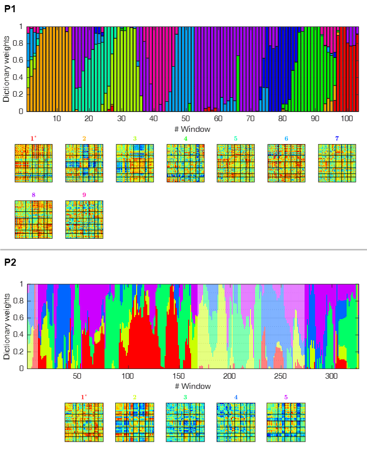
Data acquisition and pre-processing: Eight epileptic patients were studied on a 3T MRI system using an MR-compatible 32-channel EEG system (Brain Products). BOLD-fMRI (2D-EPI, TR/TE=2500/50ms) was acquired concurrently with EEG. EEG data were MR-induced artefact corrected and band-pass filtered (1-45Hz), and fMRI data were subjected to advanced pre-processing steps4. dFC was first estimated by parcelling the brain using the automated anatomical labelling (AAL) atlas, averaging the BOLD signal within each parcel, and computing the pair-wise Pearson correlation coefficient across all parcels using a sliding-window approach (window length=37.5s, step=5s)5. dFC states were then estimated using an l1-norm regularized dictionary learning approach3,6, which forces a certain degree of sparsity in time (Fig.1). Each sliding-window was labelled according to the dFC state exhibiting the highest contribution.
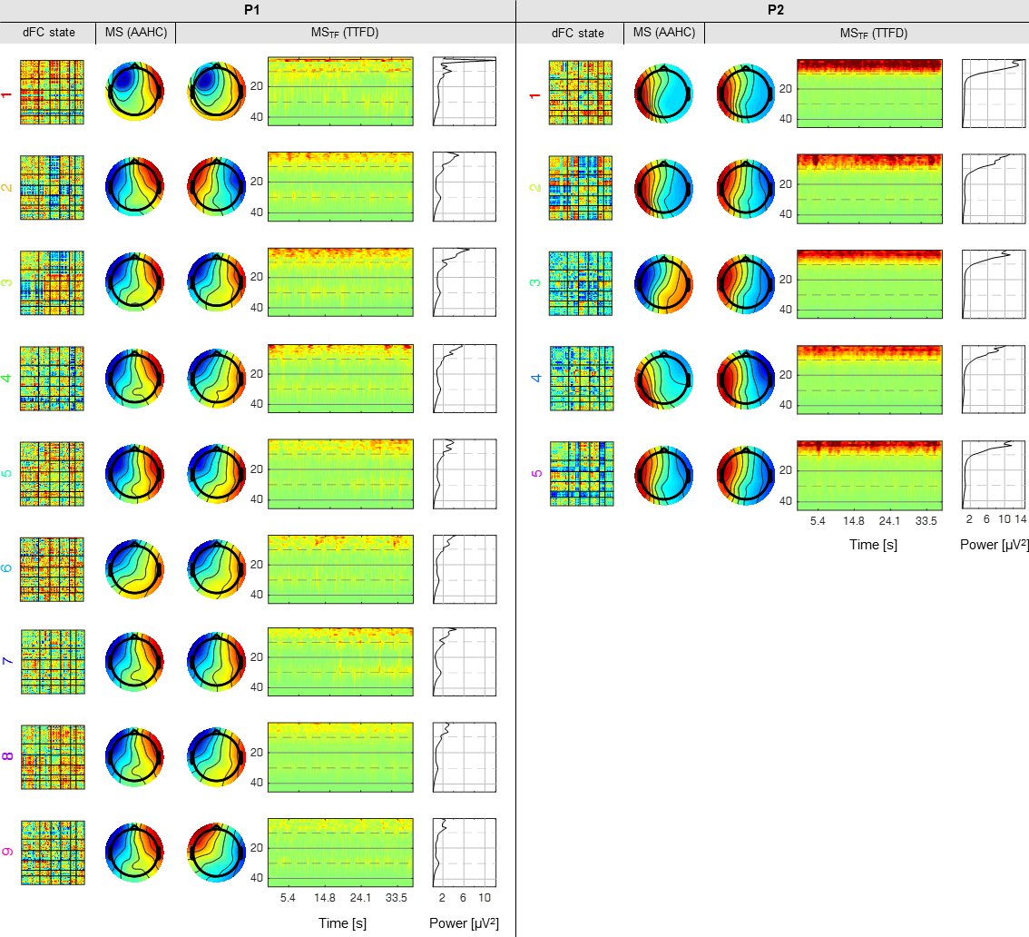
EEG microstates: Two different approaches were used to identify EEG microstates (Fig.2): atomize-agglomerative hierarchical clustering (AAHC, from an EEGLAB plug-in)7 (MS), and topographic time-frequency decomposition (TTFD)8 (MSTF). The AAHC algorithm works exclusively in the time-domain, identifying recurrent EEG topographies across those from instances of high signal-to-noise ratio as quantified by the global field power (GFP; represents the temporal standard deviation across EEG channels). TTFD first time-frequency decomposes the signal from all channels, identifies the local maxima of the GFP in the time-frequency domain, and then applies the AAHC algorithm to the associated EEG topographies. The assignment provided by AAHC was used to reconstruct the time-frequency dynamics of the resulting MSTF, from which the average spectral power (SP) over time was also computed. The number of clusters was determined as the minimum (between 3 and 6, in unit step) that explained at least 80% of the EEG variance. The variance explained by each microstate was quantified by the global explained variance (GEV)9.
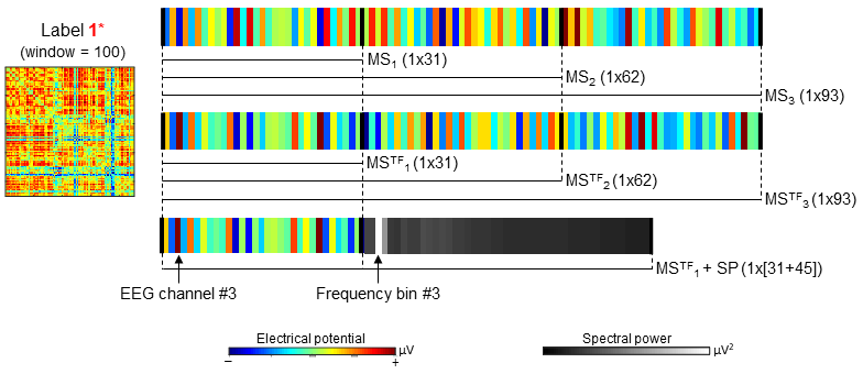
dFC state classification: Classification was carried out using random forests consisting of 50 de-correlated trees. Three models were tested for each type of microstates, based on vectorised topographies (31 channels each) with the highest (MS1/MSTF1), two highest (MS2/MSTF2) and three highest (MS3/MSTF3) GEV values. A further model comprising MSTF1 and the associated SP was also considered (31 channels+45 frequency bins), yielding a total of 7 models (illustrated in Fig.3). Bootstrapping coupled with out-of-bag samples were used to estimate the accuracy (ACC) of each model, as well as the relative importance of the EEG features (channels on MS/MSTF, and frequency bins on SP). In order to assess the possible risk of overfitting, the relative overfitting rate (ROR)10 was also computed, assuming values between 0 (no overfitting) and 1.
Results
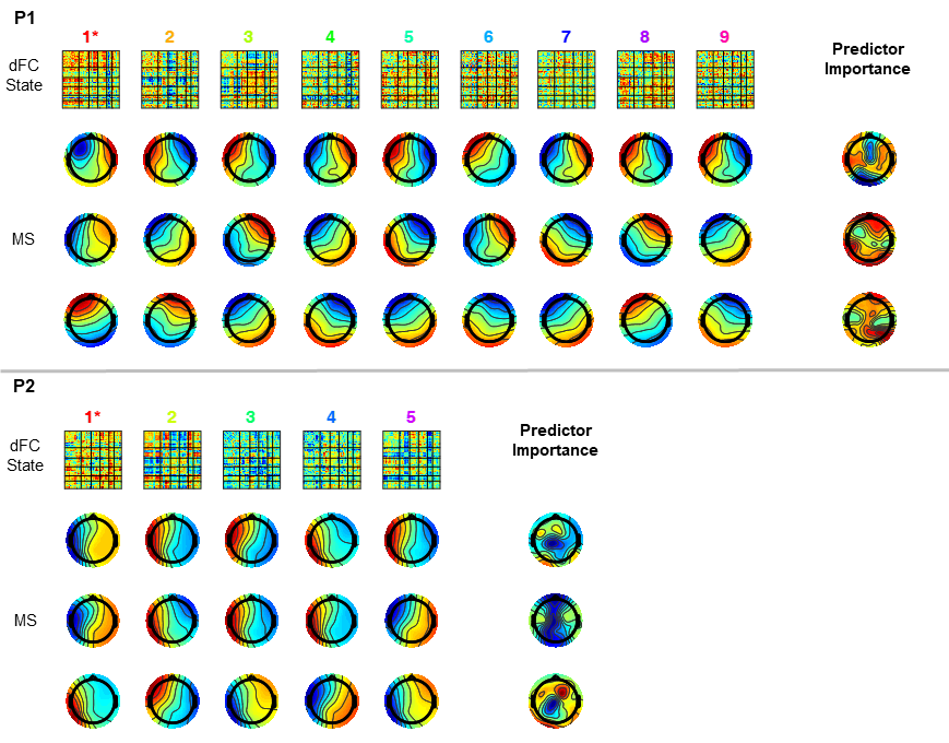
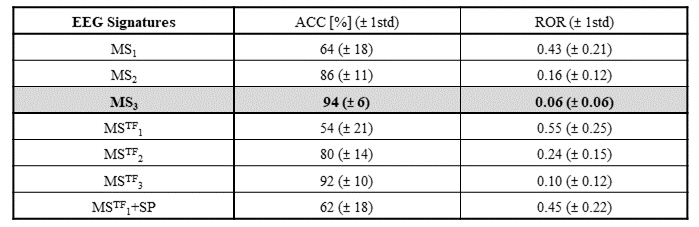
The EEG models that achieved the highest classification accuracy, together with the relative importance of each feature are shown in Fig.4, for the same two illustrative patients. For most patients (5/8), the model MS3 outperformed the remaining six in terms of ACC as well as ROR, being only surpassed by MSTF3 in the remaining patients (3/8). The average ACC and ROR values across patients are shown in Fig.5. As expected, model MS3 yielded the highest average ACC (94%) and the lowest average ROR (0.06), followed by model MSTF3 (ACC=92%, ROR=0.10). All other models yielded considerably poorer performance (ACC<90%, ROR>0.10). Moreover, these results also suggest that estimating microstates from the more complex time-frequency domain does not provide critical information for dFC state classification, as evidenced by the slightly poorer performance of the MSTF-based models.Conclusions
We showed that highly accurate classification of fMRI dFC states can be achieved based on the three EEG microstates with the highest global explained variance in simultaneous EEG-fMRI data. These results provide further support to the electrophysiological underpinnings of fMRI dFC states2,3. The existence of EEG-derived microstates correlates of fMRI-derived dFC states is also evidenced, and in agreement with those already found for fMRI-derived resting-state networks11,12. Further work is needed to extend these results to EEG-fMRI data from healthy volunteers.Acknowledgements
We acknowledge the Portuguese Science Foundation (FCT) for financial support through Project PTDC/SAUENB/112294/2009, Project PTDC/EEIELC/3246/2012 and Grant UID/EEA/50009/2013, and the POR Lisboa 2020 through Grant LISBOA-01-0145-FEDER-029675. We also acknowledge Thomas Koenig for kindly sharing the MATLAB® code of the topographic time-frequency decomposition method.
Fundação para a Ciência e Tecnologia (PEST - UID/NEU/04539/2013, COMPETE, POCI 01-0145-FEDER 007440)
References
1. Du, Y., Fu, Z. & Calhoun, V. D. Classification and Prediction of Brain Disorders Using Functional Connectivity: Promising but Challenging. Front. Neurosci. 12, 525 (2018).
2. Allen, E. A., Damaraju, E., Eichele, T., Wu, L. & Calhoun, V. D. EEG Signatures of Dynamic Functional Network Connectivity States. Brain Topogr. 1–16 (2017).
3. Abreu, R., Leal, A. & Figueiredo, P. EEG microstate and spectral signatures of epileptic patterns found in fMRI dynamic functional connectivity. in 2018 Proceedings of Joint ISMRM-ESMRMB (Joint ISMRM-ESMRMB) (2018).
4. Abreu, R., Nunes, S., Leal, A. & Figueiredo, P. Physiological noise correction using ECG-derived respiratory signals for enhanced mapping of spontaneous neuronal activity with simultaneous EEG-fMRI. Neuroimage 154, 115–127 (2017).
5. Hutchison, R. M. et al. Dynamic functional connectivity: promise, issues, and interpretations. Neuroimage 80, 360–78 (2013).
6. Mairal, J., Bach, F., Ponce, J. & Sapiro, G. Online Learning for Matrix Factorization and Sparse Coding. J. Mach. Learn. Res. 11, 19–60 (2010).
7. Delorme, A. & Makeig, S. EEGLAB: An open source toolbox for analysis of single-trial EEG dynamics including independent component analysis. J. Neurosci. Methods 134, 9–21 (2004).
8. Koenig, T., Marti-Lopez, F. & Valdes-Sosa, P. Topographic time-frequency decomposition of the EEG. Neuroimage 14, 383–390 (2001).
9. Murray, M. M., Brunet, D. & Michel, C. M. Topographic ERP analyses: A step-by-step tutorial review. Brain Topogr. 20, 249–264 (2008).
10. Hastie, T., Tibshirani, R. & Friedman, J. in The Elements of Statistical Learning 219–259 (2009).
11. Britz, J., Van De Ville, D. & Michel, C. M. BOLD correlates of EEG topography reveal rapid resting-state network dynamics. Neuroimage 52, 1162–1170 (2010).
12. Yuan, H., Zotev, V., Phillips, R., Drevets, W. C. & Bodurka, J. Spatiotemporal dynamics of the brain at rest - Exploring EEG microstates as electrophysiological signatures of BOLD resting state networks. Neuroimage 60, 2062–2072 (2012).
Figures