3729
Deriving cardiac waveforms from fMRI data using slice selective averaging and a deep learning filter.1Harvard Medical School, Boston, MA, United States, 2McLean Hospital Brain Imaging Center, Belmont, MA, United States
Synopsis
This work is a new technique to find Cardiac waveform from the fMRI data. For that purpose, a three stage data analysis is performed. In the first two stages, a candidate signal is derived by averaging over the voxels in every slice and combining them with proper time delays and resampling to 25Hz. As the third stage a deep learning architecture is used to improve the signal quality. The reconstructed signal is a good estimate of the plethysmogram data which is collected simultaneously with fMRI data.
Introduction
Cardiac waveforms, recorded simultaneously during fMRI scans, can be used for numerous purposes, including noise removal and inferring physiological state. However, cardiac waveforms are often not recorded, and are not present in many shared datasets. In this work, we develop a method to estimate the cardiac signal in the brain from the fMRI data itself. In order to achieve this, we use the following assumptions. While the individual voxel recording time (TR) is too slow to fully sample the cardiac waveform, signal from the individual slices is rapid, on the order of 10-20 Hz. Averaging the cardiac component among the slice voxels is a sufficient approximation. Individual time slice averaging can be combined with proper time delays to obtain an initial estimate for the cardiac signal. However, this signal is quite noisy and distorted. In order to de-noise the signal we use deep learning architecture to invert the signal to reconstruct the driving cardiac signal from the noisy fMRI signal estimate.Methods
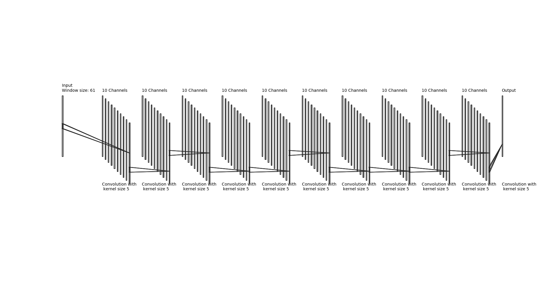
We used Human Connectome Project 1200 Subjects Release (HCP). Each HCP subject has 4 15 minute resting state acquisitions. Data was collected in 2 sessions on subsequent days, in both LR and RL phase encoding direction. We selected the first 100 subjects numerically in order to keep our training dataset manageable. We used the 400 Hz plethysmography data which was recorded simultaneously during the sessions as our ground-truth. All operations are performed on raw fMRI data prior to any preprocessing. We average the signal over all voxels for every slice (after regressing out motion timecourses and normalizing to percent deviation over time) and combine the slice timecourses with proper time delays to obtain the first raw estimate of the cardiac signal. We then resample the raw waveform to 25 Hz (to generalize the processing to work with any input sample rate). Finally, we process the raw estimate using a trained, multilayer Convolutional Neural Network (CNN) implemented in Keras to remove noise and jitter from the raw signal, yielding an improved estimate of the cardiac waveform. Network parameters are detailed in Figure 1. The network was trained on 80% of the subject data; the resampled fMRI-derived cardiac waveform was the input, the matching resampled plethysmogram data was the target. Runs with spikes in the first stage data were excluded from the training set.Results:
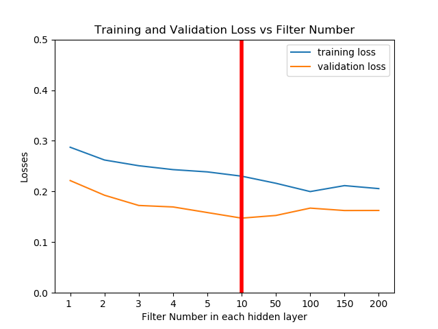
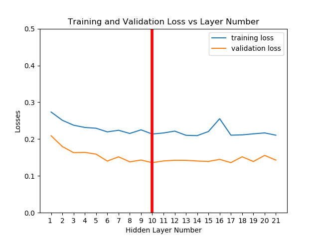
We did a simple hyper-parameter search and selected a layer depth of 10, with 10 filters of length 5 for each layer. This choice was stable and had high prediction accuracy, and a low training and computation time.
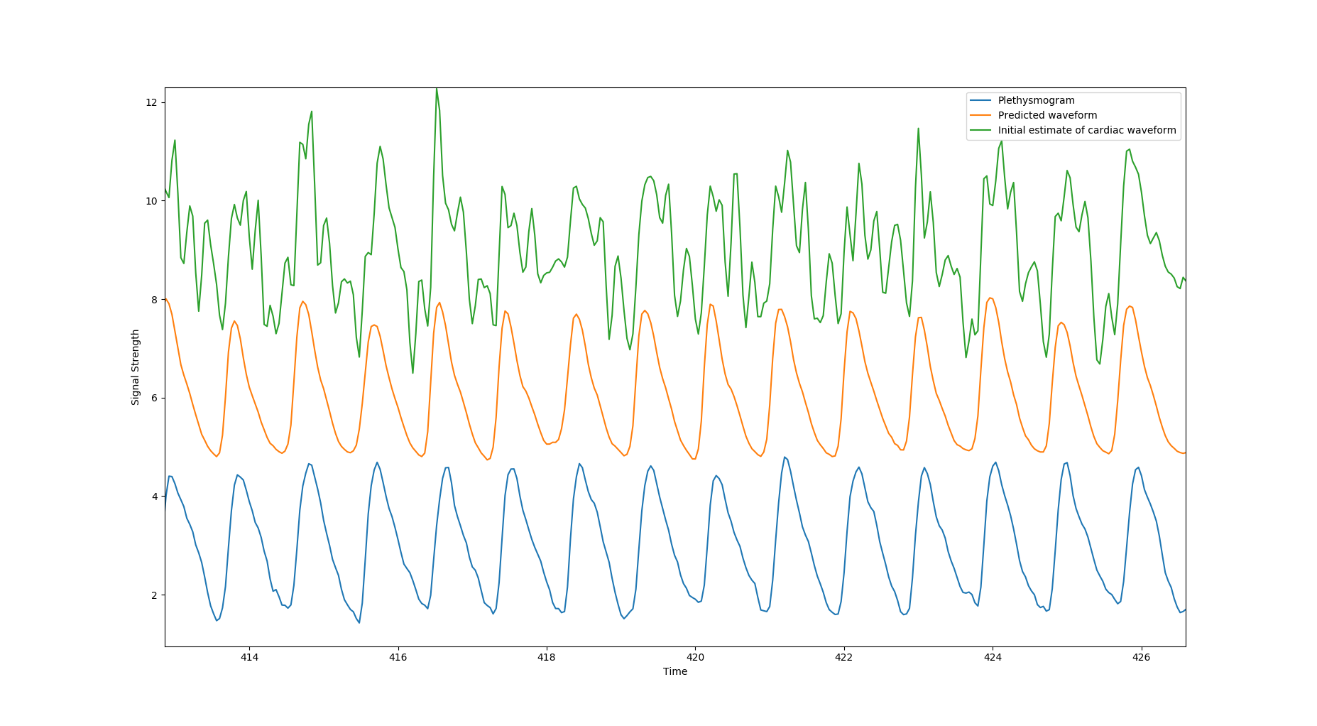
We assessed the performance in the validation set. Mean square error of Stage 2 output (raw signal) with respect to plethysmography data was 0.60. This is compared to an error of only 0.14 for the deep learning prediction (~77% noise reduction). We also tested the results by including the noisy data. In this case for the Stage 2 it is 0.86, and the deep learning prediction is 0.44.
Discussion:
The CNN noise removal filter is an extension to usual filtering approaches. In contrast to simple spectral filters, the CNN filter better recovers the waveform shape, as it incorporates prior knowledge of the structure of plethysmogram waveforms. We saw substantial improvement after applying multiple layers with multiple filters. Performance was additionally improved by regressing out motion timecourses (the 6 axis timecourses and their time derivatives). It is important to note that the data was not motion corrected, as this would move signal between slices, however the regression removed major motion correlated noise in the signals. Even with motion regression, we noticed failures in some regimes when the raw signal estimate is extremely noisy. In order to overcome this, we will explore alternative, more advanced network architectures which use global time features in the signal. We also plan to explore using phase projection results of the cardiac signals for removing cardiac noise from the fMRI signal.Conclusion:
By combining time corrected multi-slice summation of slice voxel averages with a deep learning reconstruction filter, we have successfully estimated the cardiac signal from resting state fMRI data itself. The model is trained on an existing dataset where plethysmography data was simultaneously recorded. The trained model was then tested on unseen data, and performance was found to be good, with a 77% reduction in mean squared error. The filter also worked well to reduce prediction error in spike data, despite not having been trained on it. The reconstructed cardiac signal can be used for noise removal, physiological state estimation, and analytic phase projection to construct vessel maps, even in cases where no physiological data was recorded during the scan.Acknowledgements
References
David C. Van Essen, Stephen M. Smith, Deanna M. Barch, Timothy E.J. Behrens, Essa Yacoub, Kamil Ugurbil, for the WU-Minn HCP Consortium. (2013). The WU-Minn Human Connectome Project: An overview. NeuroImage 80(2013):62-79.Figures