3646
Kärger Model Difficulties for In Vivo DWICatherine L Lian1,2, Brendan Moloney2, Eric M Baker2, Greg Wilson3, Erin W Gilbert4, Thomas M Barbara2, Charles S Springer2, and Xin Li2
1Westview High School, Portland, OR, United States, 2Advanced Imaging Research Center, Oregon Health & Science University, Portland, OR, United States, 3Home, Mill Creek, WA, United States, 4Surgery, Oregon Health & Science University, Portland, OR, United States
Synopsis
Although it is well known that diffusion-weighted imaging (DWI) is sensitive to in vivo trans-membrane water-exchange, quantitative interpretation of the diffusion b-space decay remains difficult. Using random-walk simulated DWI data, this study investigates the feasibility and reliability in studying the water exchange effects with a multi-exponential fitting approach on DWI data.
Purpose
Diffusion-weighted imaging (DWI) is sensitive to in vivo trans-membrane water-exchange. However, quantitative interpretation of the diffusion decay remains difficult. Recent Inverse Laplace Transformations1 of DWI data spanning up to b values of 6000 s/mm2 showed only one diffusigraphic peak for each brain tissue type (grey matter, white mater, etc.). Using [random-walk] RW-simulated DWI data, the purpose of this study is to investigate the feasibility and reliability in studying the water exchange effects on DWI using a multi-exponential fitting approach.Method
A Monte Carlo [MC] RW approach is used to simulate DWI data.2 Water molecule displacements within a 3D ensemble of 10,648 identical spheres having hexagonal close-packed symmetry are simulated. The 37 oC pure water diffusion coefficient, D0 = 3.0 μm2/ms, is used for all particles, whether inside or outside cells. Noise-free in silico DWI decay curves for five steady-state cellular water efflux exchange rate constant (kio) values of 0, 2, 4, 6, 10 (s-1) are generated.Results
Figure 1a and 1b show simulated DWI b-space decay points with kio = 0 [above] and 10 s-1 [below]. Blue and red curves show empirical single- (a) and biexponential (b) fittings of the kio = 0 and 10 points, respectively. Based on the Akaike information criterion (AIC), each of the five noiseless data sets is better fitted by a bi-exponential model [only two are shown in Fig. 1a and in 1b]. When the natural logs of the simulated data are plotted against b-values (Fig. 1c), none of the five decays exhibit a straight line. The AIC model selection outcome could change quickly with increasing Gaussian noise present in the data. Using MC simulations, Figure 2 shows the fractions of fittings for which a biexponential model is favored, for three different SNR values: 50, 15, 5. The five bars from left to right for each SNR represent the five kio values of 0, 2, 4, 6, 10 s-1 , respectively. When SNR diminishes to 5, there is no clear exponentiality preference.Discussion
Multi-exponential fitting has been used extensively in DWI and the two-site exchange Kärger model3 has been frequently adapted for in vivo MRI. However, quantitative interpretation remains controversial. Conflicting literature results could partially arise from different study designs. Besides the SNR effects mentioned above, inter-compartmental water exchange issues can be visualized with Figure 3. It plots system rate constants vs. b-values. Line AC measures the overall exchange rate constant [k = kio + koi ], where koi is cellular water influx rate constant. Line OAB traces the maximum “diffusigraphic shutter-speed,” кD , defined as |qmax2ΔD|,4 where ΔD is (D2 - D1 ), the site ADC difference, and qmax is the maximum q value achieved during the b variation: b is changed by incrementing q with fixed diffusion time, Δ. Line BC indicates the diffusion-weighting with highest b-value achieved at qmax2. For a reliable exchange-sensitive bi-exponential fitting, кD has to be sufficiently greater than k.4 Practically, this means some DWI data points have to be measured with |q2ΔD| values above the horizontal AC line. Thus, ABC represents a “golden triangle” to facilitate water exchange measurement using the Kärger model.3 To maximize water exchange-sensitivity, the more points inside the golden triangle the better. Unlike DCE-MRI, the degree of exchange-sensitivity in the DWI experiment is somewhat under the operator’s control. For the same b value, a pulse sequence with higher q2 is more sensitive to water exchange than the one with smaller q2. One exchange-insensitive example is shown by line OD, where no experimental points could reach the golden triangle due to a qmax that is too small. The common practice of achieving large b-values by increasing Δ can often lead to sub-optimal qmax. It also becomes obvious that for systems with negligible ΔD values, as implied for the human brain,1 attempts to extract water exchange and ADCs from bi-exponential fittings are likely to be unsuccessful. For the current study, a qmax value of ~51.9 mm-1 is achieved at maximum b-value of 4600 s/mm2. With an estimated ΔD of ~ 1.3 μm2/ms, the maximum кD achieved is 3.5 s-1, which is smaller than the overall exchange rate for almost all non-zero kio cases. Therefore, the simulation for a typical clinical DWI study doesn’t reach the sufficiently large кD required. If the Kärger model is used, a single exponential decay would generally be expected, especially with faster overall exchange rate. Other factors, like non-single-valued ADCs within each compartment, may contribute to outcomes where multi-exponentiality is AIC-preferred even for SNRs as low as 10 (Figure 2). A different DWI approach2 determines k when кD = 0.Acknowledgements
NIH: R44 CA180425, OHSU Brenden-Colsen Center for Pancreatic Care.References
1. Avram, Sarlls, Basser, PISMRM, 26:5242 (2018). 2. Springer, Wilson, Moloney, Barbara, Li, Rooney, Maki, PISMRM 26:261 (2018). 3. Kärger, Adv.Colloid. Interfac. 23:129–148 (1985). 4. Lee, Springer, MRM, 49:450–458 (2003).Figures
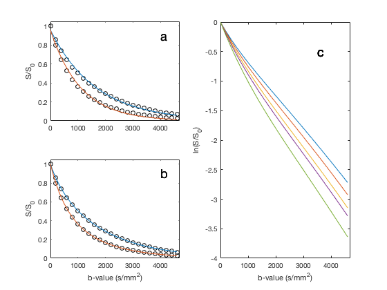
Figure 1: a and b. The circles show simulated DWI data with kio of 0 and 10 s-1, above and below, respectively. Solid curves show empirical single exponential (a) and biexponential (b) fittings, red and blue, respectively, of the simulated data. Based on the Akaike information criterion (AIC), all five noiseless data sets can be better fitted by a biexponential model. When the natural logs of the simulated data are plotted against b-values (c), none of these show a perfect straight line.
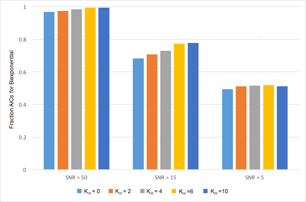
Figure 2. With Gaussian noise being the only difference in each run, the fractions of fittings that favor the biexponential models under three SNR values of 50, 15, 5 are shown. The five bars from left to right represent the five kio values of 0, 2, 4, 6, 10 s-1, respectively. When SNR has diminished to 5, no clear preference is indicated for either model.
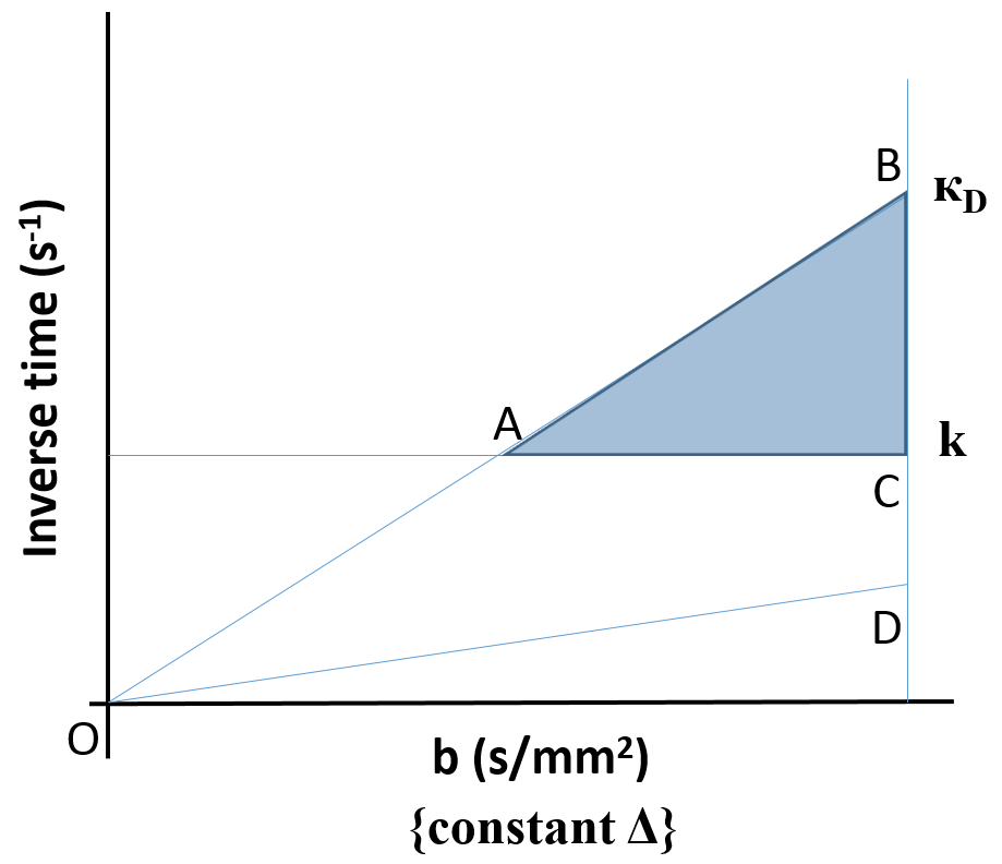
Figure 3: A cartoon plot of DWI sensitivity to water exchange with increasing b values. Line AC measures the overall exchange rate constant [k = kio + koi], Line OAB traces the maximum “diffusigraphic shutter-speed,” кD, defined as |qmax2ΔD|. Line BC indicates the diffusion-weighting with highest b-value achieved at qmax2. Under fixed Δ condition, all DWI data points will be on or below the OAB line. To maximizing the sensitivity of DWI data to water-exchange, the more points within the “golden triangle”, ABC, the better.