3584
Joint distribution of axonal length and diameter quantifies beading in traumatic brain injury1National Institutes of Health, Bethesda, MD, United States, 2Center for Neuroscience and Regenerative Medicine, Bethesda, MD, United States
Synopsis
We present a novel diffusion MRI approach to measure the three-dimensional axonal morphology alterations following traumatic brain injury that results in beading, by modeling axons with a two-dimensional joint distribution of diameters and lengths ($$$D$$$-$$$L$$$). Here we study a segment of ferret spinal cord tissue with known and focal Wallerian degeneration of the corticospinal tract alongside an uninjured control. The results suggest that this approach can be used to specifically detect and quantify axonal beading.
Introduction
Axonal beading is a primary result of white matter (WM) injury following brain and spinal cord trauma that can reverse or can progress to neuronal degradation.1,2 Noninvasive imaging tools that can detect this pathology could be used to monitor the progression of axonal recovery or degeneration. Diffusion MRI is a promising candidate for this purpose owing to its high sensitivity to microstructural changes.3 However, models such as diffusion tensor imaging (DTI)4 may not provide the needed specificity to detect subtle changes in WM beading such as the size distribution of the beads or their spacing. Due to the nature of the three-dimensional alterations in axon morphology following trauma, it was hypothesized that characterizing beading using a two-dimensional joint distribution of diameters and lengths of finite axonal segments ($$$D$$$-$$$L$$$) could potentially detect this type of injury.5 It was also shown that a three-dimensional double diffusion encoding (DDE) acquisition (Fig. 1), coupled with constrained optimization, could be used to reconstruct the joint $$$D$$$-$$$L$$$ distribution nonparametrically in WM.5 Here, we applied this experimental and modeling pipeline to study a segment of ferret spinal cord tissue with known and focal Wallerian degeneration of the corticospinal tract (CST) alongside an uninjured control to determine whether axonal beading could be reliably and specifically detected.Methods
Two perfusion fixed ferret spinal cord specimens were obtained from tissue collected as part of a larger study.6 One from an uninjured control and the other from a ferret that underwent closed head injury resulting in focal hemorrhage of the CST at the level of the caudal brainstem. No direct injury was observed in the segment of spinal cord used in this study. Wallerian degeneration was expected along the CST region of the specimen, but not others. Exploiting the separation of displacement variables in the parallel and perpendicular directions within the capped cylinder model,7 we acquired DW data according to the schemes in Figs. 1 and 2, and processed the data according to a constrained optimization framework suggested elsewhere.5,8 This approach provides a marginal axon diameter distribution (MADD), a marginal axon length distribution (MALD), and their joint $$$D$$$-$$$L$$$ distribution in each imaging voxel.
Results and Discussion
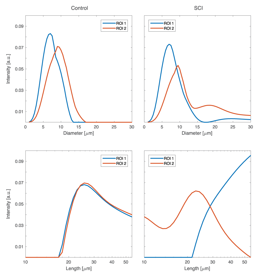
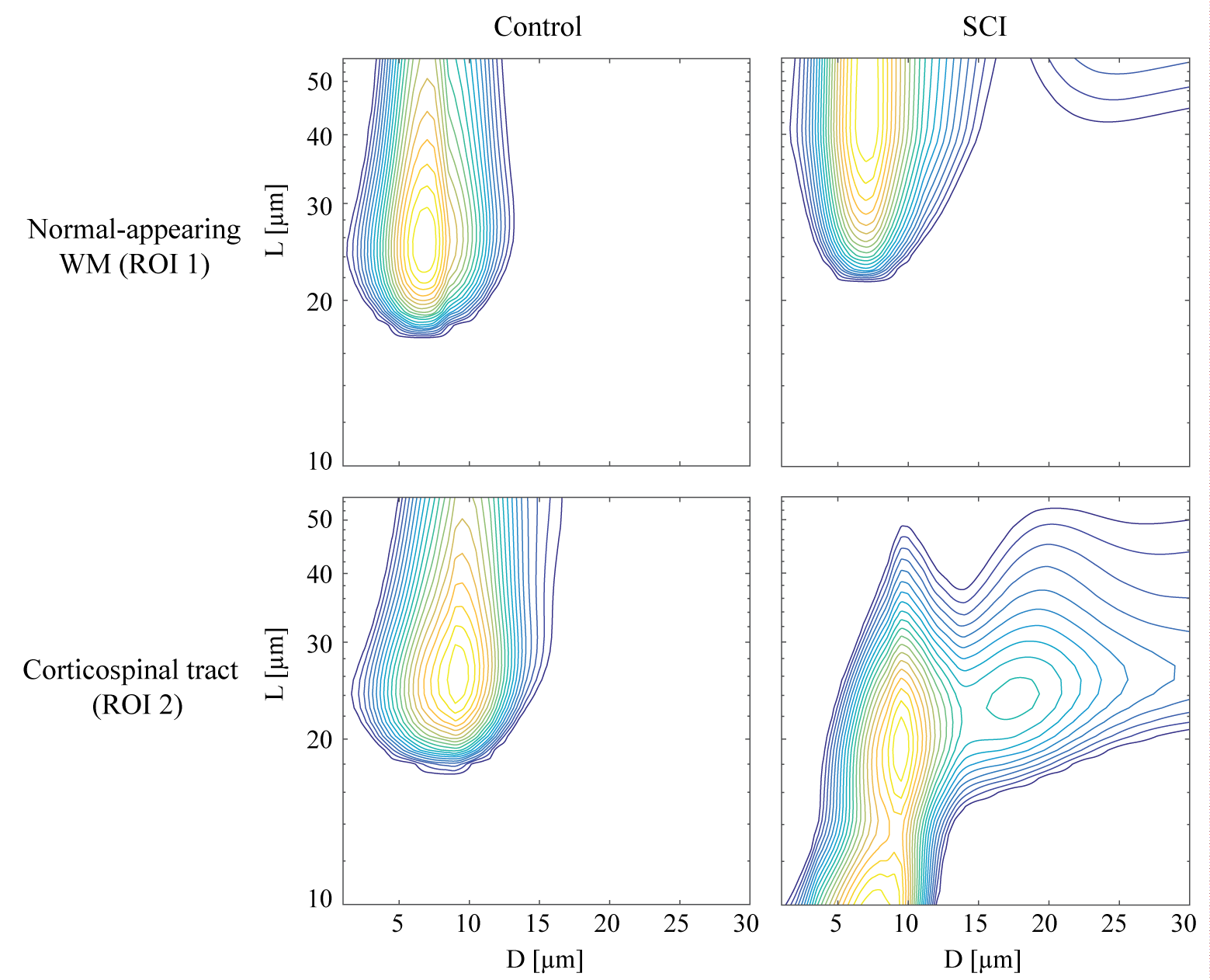
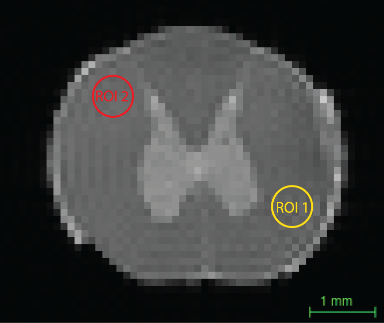
In this study, we chose to focus on a single slice of the spinal cord, and on two regions of interest (ROI): normal-appearing WM and the spinal cord injury (SCI) region, CST, which were marked as ROIs 1 and 2, respectively, in Fig. 2. First, the 1D marginal distributions, MADD and MALD were obtained from both ROIs in both of the control and SCI specimens. These spectra are shown in Fig. 3. First examining the control sample, the MADDs appear unimodal, with ROI 2 having a slightly shifted distribution, compared to ROI 1. For the axon length distribution, both ROIs have very similar MALDs. A long tail at larger $$$L$$$ values is expected in the case of healthy WM tissue because of the increased validity of the infinite cylinder model. Conversely, in the SCI sample both the MADD and the MALD have very different features in the normal-appearing WM and the CST ROIs. The injury resulted in a second peak with larger diameters in the diameter distribution spectrum. This peak may have originated from the beaded axon population. In the longitudinal plane, the difference is even more pronounced, and the MALD of the injury site is more peaked at the low-end of the spectrum, which can be attributed to the expected narrowing of the axons due to beading. The 2D joint $$$D$$$-$$$L$$$ distributions from the control and SCI samples are shown in Fig. 4. With the exception of the CST ROI from the SCI sample, it is evident that in all other cases the $$$D$$$-$$$L$$$ spectra were qualitatively similar, with most of the spectral energy concentrated at the large $$$L$$$ and small $$$D$$$ regions. The CST $$$D$$$-$$$L$$$ spectrum from the injured sample was markedly different, with the majority of the spectral intensity appearing in the lower-medium $$$L$$$ range. These results demonstrate that modeling axons as an ensemble of parallel finite capped cylindrical pores provides three-dimensional microstructural information that reflects axonal beading.Conclusion
We showed here how MRI can be used to quantify the three-dimensional WM microstructure using a novel $$$D$$$-$$$L$$$ spectrum. The unique information contained in these spectra may provide a long-sought after increase in specificity to microscopic microstructural alterations in white matter that follow traumatic brain injury. The combination of measuring a $$$D$$$-$$$L$$$ spectrum with spatial localization could provide a means to measure and map axonal or nerve injury within the CNS and PNS, respectively.Acknowledgements
This work was supported by the Intramural Research Program of the Eunice Kennedy Shriver National Institute of Child Health and Human Development [grant numbers HD000266] and The Henry M. Jackson Foundation for the Advancement of Military Medicine, Inc., [HJF Award Numbers: 308049-8.01-60855 and 307513‐3.01‐60855].References
- Johnson V, Stewart W, Smith D. Axonal pathology in traumatic brain injury. Experimental Neurology. 2013;246:35-43.
- Ochs S, Pourmand R, Jersild RA, et al. The origin and nature of beading: a reversible transformation of the shape of nerve fibers. Progress in Neurobiology. 1997;52:391-426.
- Budde MD, Frank JA. Neurite beading is sufficient to decrease the apparent diffusion coefficient after ischemic stroke. Proc Natl Acad Sci USA. 2010;107:14472-14477.
- Basser PJ, Mattiello J, LeBihan D. MR diffusion tensor spectroscopy and imaging. Biophysical Journal. 1994;66:259-267.
- Benjamini D, Basser PJ. Joint radius-length distribution as a measure of anisotropic pore eccentricity: An experimental and analytical framework. The Journal of Chemical Physics. 2014;141:214202.
- Hutchinson EB, King SG, Kim Y, et al. MRI markers of brain injury in a ferret model of closed head rotation and acceleration. 2018 Society for Neuroscience, San Diego, CA.
- Ozarslan E. Compartment shape anisotropy (CSA) revealed by double pulsed field gradient MR. Journal of Magnetic Resonance. 2009;199:56-67.
- Benjamini D, Basser PJ. Use of marginal distributions constrained optimization (MADCO) for accelerated 2D MRI relaxometry and diffusometry. Journal of Magnetic Resonance. 2016;271:40-45.
Figures
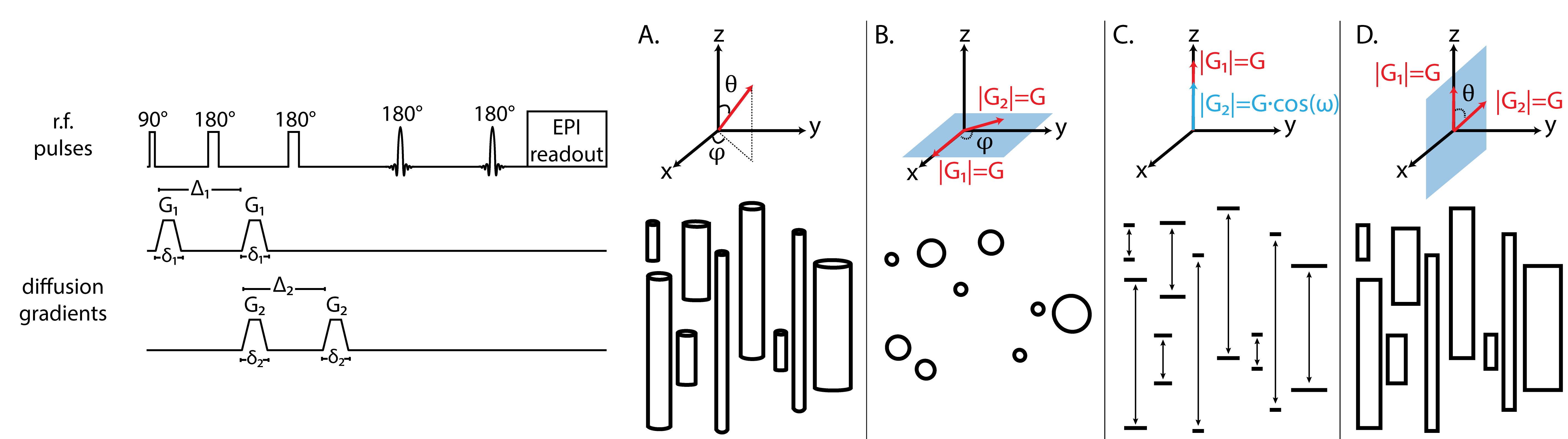
MRI data were collected on a 7 T Bruker wide-bore vertical magnet using a 3D EPI DDE sequence according to the scheme in Fig. 1. The parameters were: (1) transverse plane: six gradient steps within $$$300-673$$$ mT/m, 12 $$$\varphi$$$ steps within $$$0-330^{\circ}$$$. (2) longitudinal plane: five gradient steps within $$$75-225$$$ mT/m, 13 $$$\omega$$$ steps within $$$0-180^{\circ}$$$. (3) joint plane: five gradient steps within $$$75-225$$$ mT/m, 12 $$$\theta$$$ steps within $$$0-330^{\circ}$$$. In all cases, gradient duration, $$$\delta_1=\delta_2=3 ms$$$ and separation, $$$\Delta_1=\Delta_2=30 ms$$$, were used, $$$TR=700 ms$$$, $$$TE=24 ms$$$, with a $$$100 \mu m$$$ isotropic resolution, with four averages and four segments.