3549
Time Dependence in B-Tensor Encoding1Centre for Medical Image Computing, University College London, London, United Kingdom, 2Great Ormond Street Institute of Child Health, University College London, London, United Kingdom
Synopsis
B-tensor encoding is becoming increasingly popular in microstructural imaging. In this technique microscopic tissue features are estimated by using different gradient waveforms that typically have different time regimes. This work studies for the first time two potential time-dependence issues that arise from these methods in-vivo in the human brain. We detect time-dependence effects in both cases, and even though these are small on a clinical system, they should not be overlooked.
Introduction
B-tensor encoding is a diffusion MRI technique that provides measurements of higher specificity to tissue heterogeneity and microscopic anisotropy than conventional diffusion methods. This is achieved by comparing signal decay from different types of diffusion encoding, commonly spherical tensor encoding (STE) and linear tensor encoding (LTE)1,2.
By combining these different sequences, B-tensor encoding assumes that diffusion is Gaussian within microscopic compartments and does not depend on time. This is not true in tissue, as cellular structures hinder diffusion and make the apparent diffusion coefficient dependent on the spectral content of the gradient waveform3-5. In this work we identify two sources of time-dependence in B-tensor encoding and investigate the effect of these in-vivo in the brain:
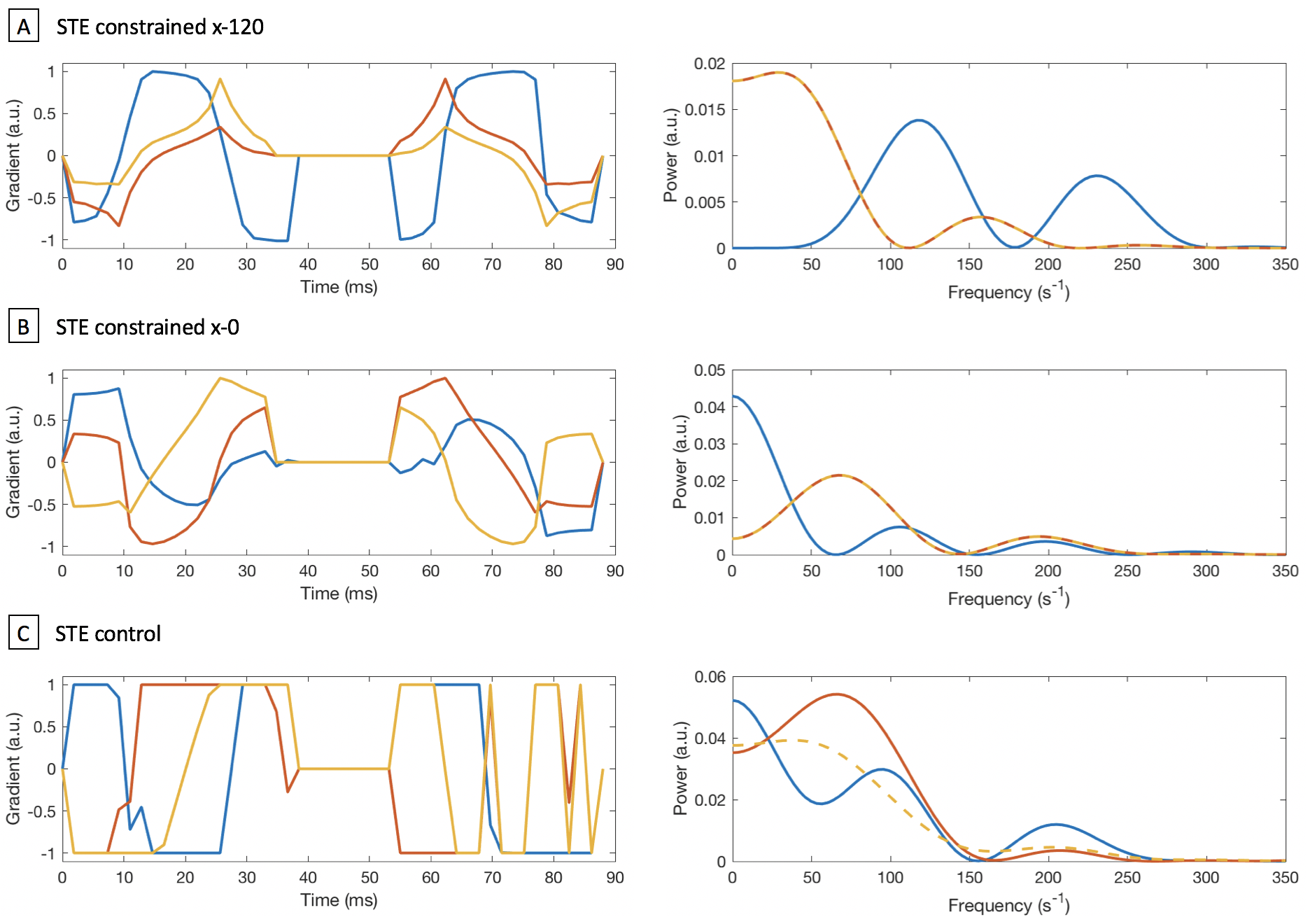
(i) STE is designed to be isotropic. However, the spectral content of the x, y and z-axes of the gradient waveform is typically not isotropic (Fig 1). Here we study whether time-dependence makes diffusion encoding through STE anisotropic in clinical measurements.
(ii) Once the STE sequence is designed, it is not obvious how to design the corresponding LTE waveform. We study the influence of the choice of LTE waveform on the diffusion attenuated signal and estimated microscopic fractional anisotropy.
Methods
Healthy volunteers and a phantom with isotropic diffusivity were scanned on a 3T Siemens Prisma scanner using a 64-channel head coil. Diffusion waveforms were designed using Maxwell compensation6,7.
(i) Time-dependence within STE
For this study, one LTE and three different STE waveforms were designed. Figure 1 shows that in two STE waveforms, the power spectra of the y and z-axes were constrained to be the same. The largest peak of the x-axis is centred around 120 s-1 in Figure 1A, and around 0 s-1 in Figure 1B. In the third STE waveform, STE control (Fig 1C), all three power spectra are similar. The waveforms were rotated so that the x-axis sampled 60 uniformly distributed gradient directions. In each case, b=2000 s/mm2, TE=106 ms and TR=8.3 s.
(ii) Time-dependence between STE and LTE
In this study, STE was measured with two LTE designs inspired by previous work8, ‘LTE-detuned’ and ‘LTE-tuned’. LTE-detuned is the magnitude of all three STE axes projected onto a single axis, while LTE-tuned is a single coordinate in STE (Fig 2). B-values of [0, 100, 500, 1000, 1500, 2000] s/mm2 were measured for each waveform with TE=99 ms and TR=8.3 s.
Results and Discussion
(i) Time-dependence within STE
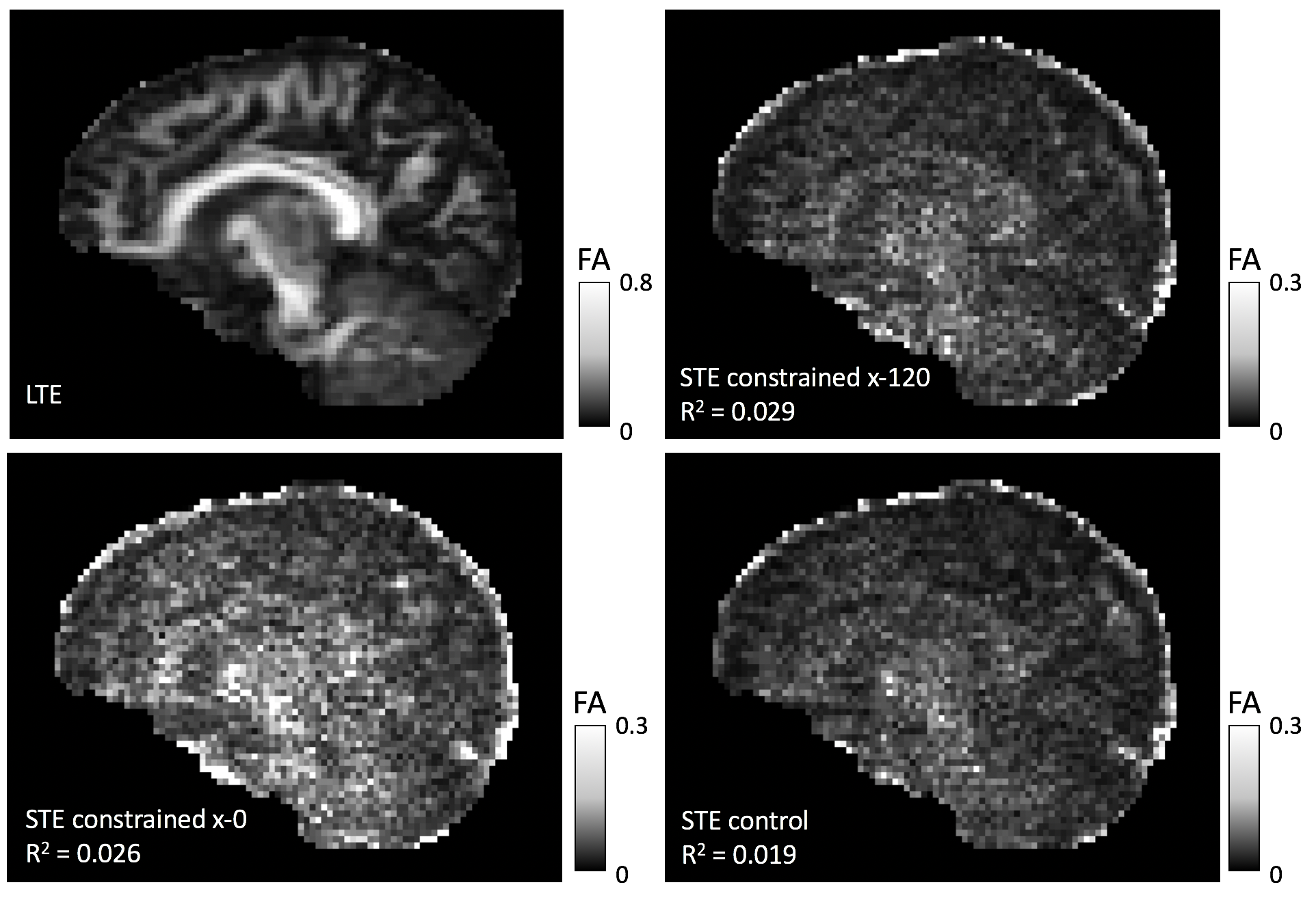
To determine whether time-dependence influences STE, the macroscopic diffusion tensor was calculated for each STE and the LTE waveform. Two parameters are compared: FA and the principal diffusion direction. If STE is truly isotropic, it does not encode directional information and FA is expected to be zero. Figure 3 shows FA maps with R2-correlation coefficients between LTE and each STE. FA is lower in STE than in LTE, but the values are slightly correlated. STE control has the lowest correlation, which suggests a time-dependence effect in the two constrained STE waveforms.
The angle between the principal diffusion directions estimated from LTE and the different STE waveforms were computed for FALTE>0.5. Figure 4 shows the distributions of angles compared to a random distribution, along with p-values obtained from a two-sample Kolmogorov-Smirnov test. The low p-values indicate that the diffusion directions obtained from STE are not random. STE control is the closest to a random distribution, which again demonstrates the influence of time-dependence.
(ii) Time-dependence between LTE and STE
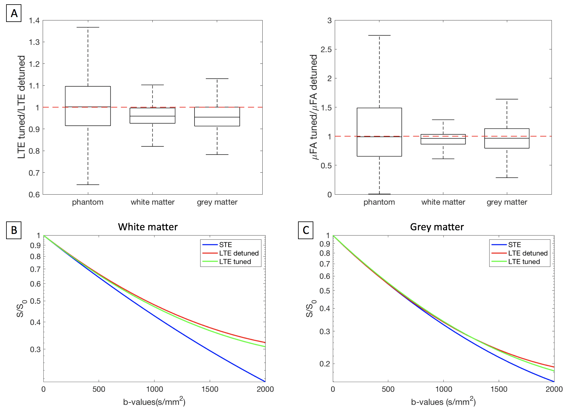
To determine whether the choice of LTE influences in-vivo results in B-tensor encoding, the signal at b=2000 s/mm2 and estimated μFA values are compared for LTE-tuned and detuned in the brain and in a phantom. Figure 5 shows that both the signal and estimated μFA is lower in LTE-tuned than in LTE-detuned. For the phantom, the ratio of signals and μFA are 1, which rules out measurement artefacts. The ratio of signals is 0.95 for both white and grey matter, and the ratio of μFA is 0.96 for both white and grey matter, which indicates that there is a time-dependence effect related to LTE design.
Conclusion
We detect time-dependence effects in B-tensor encoding, both within the STE waveform and in the design of LTE. The effect in STE is shown for the first time, and results in LTE are similar to those shown by Lundell8 in ex-vivo monkey brain. Although the effect is small in clinical settings, we believe it should not be completely ignored as it has in most past work. For STE, the time-dependence effect may be reduced by rotating the waveform and powder-averaging the signal. The question of how to design LTE is open and should be studied in future work.Acknowledgements
The authors thank the London Interdisciplinary Bioscience PhD Consortium and the following grants for funding: BBSRC BB/M009513/1, UK EPSRC EP/M020533/1, EP/N018702/1 and EU H2020 634541-2. We also thank Filip Szczepankiewicz and Markus Nilsson for sharing their free-waveform diffusion EPI sequence.References
[1] Lasic, S., Szczepankiewicz, F., Eriksson, S., Nilsson, M., Topgaard, D. (2014), Microanisotropy imaging: quantification of microscopic diffusion anisotropy and orientational order parameter by diffusion MRI with magic-angle spinning of the q-vector. Frontiers in Physics, 2: 11.
[2] Szczepankiewicz, F., Lasic, S., van Westen, D., Sundgren, P. C., Englund, E., Westin, C.-F., Stahlberg, F., Latt, J., Topgaard, D., Nilsson, M. (2015), Quantification of microscopic diffusion anisotropy disentangles effects of orientation dispersion from microstructure: Applications in healthy volunteers and in brain tumors. NeuroImage, 104, 241-252.
[3] Stepisnik, J. (1981), Analysis of NMR self-diffusion measurements by a density matric calculation. Physica B+C, 104:3, 350-364.
[4] Grebenkov, D. S. (2010), Use, misuse, and abuse of apparent diffusion coefficients. Concepts in Magnetic Resonance, 36A: 24-35.
[5] Jespersen, S. N., Lundell, H., Sonderby, C. K., Dyrby, T. B. (2014), Commentary on “Microanisotropy imaging: quantification of microscopic diffusion anisotropy and orientation of order parameter by diffusion MRI with magic-angle spinning of the q-vector. Frontiers in Physics, 2, 28.
[6] Sjolund, J., Szczepankiewicz, F., Nilsson, M., Topgaard, D., Westin, C. F., Knutsson, H. (2015), Constrained optimization of gradient waveforms for generalized diffusion encoding. Journal of Magnetic Resonance, 261, 157-168.
[7] Szczepankiewicz, F., Nilsson, M. (2018), Maxwell-compensated waveform design for asymmetric diffusion encoding, ISMRM 2018, Paris, France.
[8] Lundell, H., Nilsson, M., Bjorn Dyrby, T., Parker, G. J. M., Hubbard Cristinacce, P. L., Zhou, F., Topgaard, D. and Lasic, S. (2017), Microscopic anisotropy with spectrally modulated q-space trajectory encoding, ISMRM 2017, Honolulu, HI, USA.
Figures