3541
HOTmix: characterizing hindered diffusion using a mixture of generalized higher order tensors1Signal Processing Lab (LTS5), Ecole Polytechnique Fédérale de Lausanne, Lausanne, Switzerland, 2Danish Research Center for Magnetic Resonance, Copenhagen University Hospital Hvidovre, Hvidovre, Denmark, 3Department of Radiology, University Hospital Center, Lausanne, Switzerland, 4ICTEAM, Université catholique de Louvain, Louvain-la-Neuve, Belgium, 5Department of Radiology, University Hospital Center and University of Lausanne, Lausanne, Switzerland, 6Department of Computer Science, University of Verona, Verona, Italy, 7Department of Applied Mathematics and Computer Science, Technical University of Denmark, Kongens Lyngby, Denmark
Synopsis
We present HOTmix, a new model to describe the diffusion MRI signal for molecules undergoing hindered diffusion. HOTmix is based on a mixture of generalized higher order tensors, explicitly incorporating the diffusion sequence’s time-dependent parameters. The method was evaluated on simulated diffusion MRI signals obtained through Monte Carlo simulations, using intermediate diffusion times, mimicking both ex-vivo and in-vivo conditions. HOTmix provided better reconstructions compared to the standard diffusion tensor, the kurtosis tensor, and a single generalized higher order tensor. In future work, we will explore whether modelling the hindered compartment using HOTmix improves microstructural features estimated using dMRI.
Introduction
Diffusion MRI (dMRI) allows estimating White Matter (WM) microstructural features in-vivo and ex-vivo, by using compartment models to characterize restricted and hindered components. Methods usually rely on a diffusion tensor (DT) to characterize the hindered comparment.1,2,3 At long diffusion times, including time dependence in the DT formulation has improved axon diameter estimates.4 Optimized protocols for diameter estimation rely on intermediate diffusion times (dozens of milliseconds).2,5 For this purpose, we propose to model the hindered compartment using HOTmix, a mixture of generalized higher order tensors (HOT).6Theory
If the WM is modeled as parallel cylinders, the HOT tensor6 becomes axi-symmetric. We found its signal to be:$$\frac{S}{S_0}=e^{-b^{(2)}D_\parallel^{(2)}cos^2(\alpha)-b^{(2)}D_\perp^{(2)}sin^2(\alpha)+b^{(4)}D_\perp^{(4)}sin^4(\alpha)}$$where $$$b^{(n)}=-(\gamma G\delta)^n(\Delta-\frac{n-1}{n+1}\delta)$$$ (G, $$$\Delta$$$ and $$$\delta$$$ are the gradient amplitude, separation and duration, respectively),6 $$$\alpha$$$ is the angle between the diffusion gradient and axon orientations, and $$$D_\parallel^{(n)}$$$ and $$$D_\perp^{(n)}$$$ are the n-th order parallel and perpendicular diffusivities. $$$b^{(n)}$$$ has a time-dependent term that differs from $$$(b^{(2)})^n$$$, used in the kurtosis tensor (KT) for example. HOTmix assumes that different spin packets experience different local micro-environments, each generating a signal given by an axi-symmetric HOT:$$\frac{S}{S_0}=\iint P(D_\perp^{(2)},D_\perp^{(4)}) e^{-b^{(2)}D_\parallel^{(2)}cos^2(\alpha)-b^{(2)}D_\perp^{(2)}sin^2(\alpha)+b^{(4)}D_\perp^{(4)}sin^4(\alpha)}dD_\perp^{(2)}dD_\perp^{(4)}$$The equation can be linearized to $$$S/S_0 = Aw$$$,7 were $$$A$$$ is a matrix containing columns $$$A_i=e^{-b^{(2)}D_{i,\parallel}^{(2)}cos^2(\alpha)-b^{(2)}D_{i,\perp}^{(2)}sin^2(\alpha)+b^{(4)}D_{i,\perp}^{(4)}sin^4(\alpha)}$$$ and $$$w_i$$$ are the relative contribution of each column to the total signal. The orientation is estimated from the DT 1st eigenvector,7 and $$$D_\parallel^{(2)}$$$ taken from the DT 1st eigenvalue. The coefficients $$$w$$$ are estimated by minimizing the following problem:$$argmin_{w \geq 0}||Aw-S||_2^2$$Matching the axi-symmetric HOT model with the signal of a gaussian distribution of diffusivities,8 our model can be interpreted as a mixture of gaussians with time-varying variance:$$P(D_\perp)=\sum_i\mathcal{N}\left(\mu=D_{i,\perp}^{(2)},\sigma^2=2D_{i,\perp}^{(4)}\frac{(\Delta-\frac{3\delta}{5})}{(\Delta-\frac{\delta}{3})^2}\right)$$which goes in line with the coarse-graining illustration for dMRI.9Methods
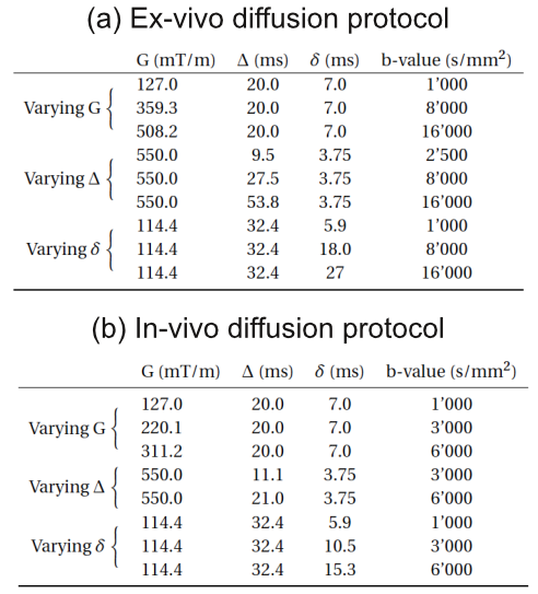
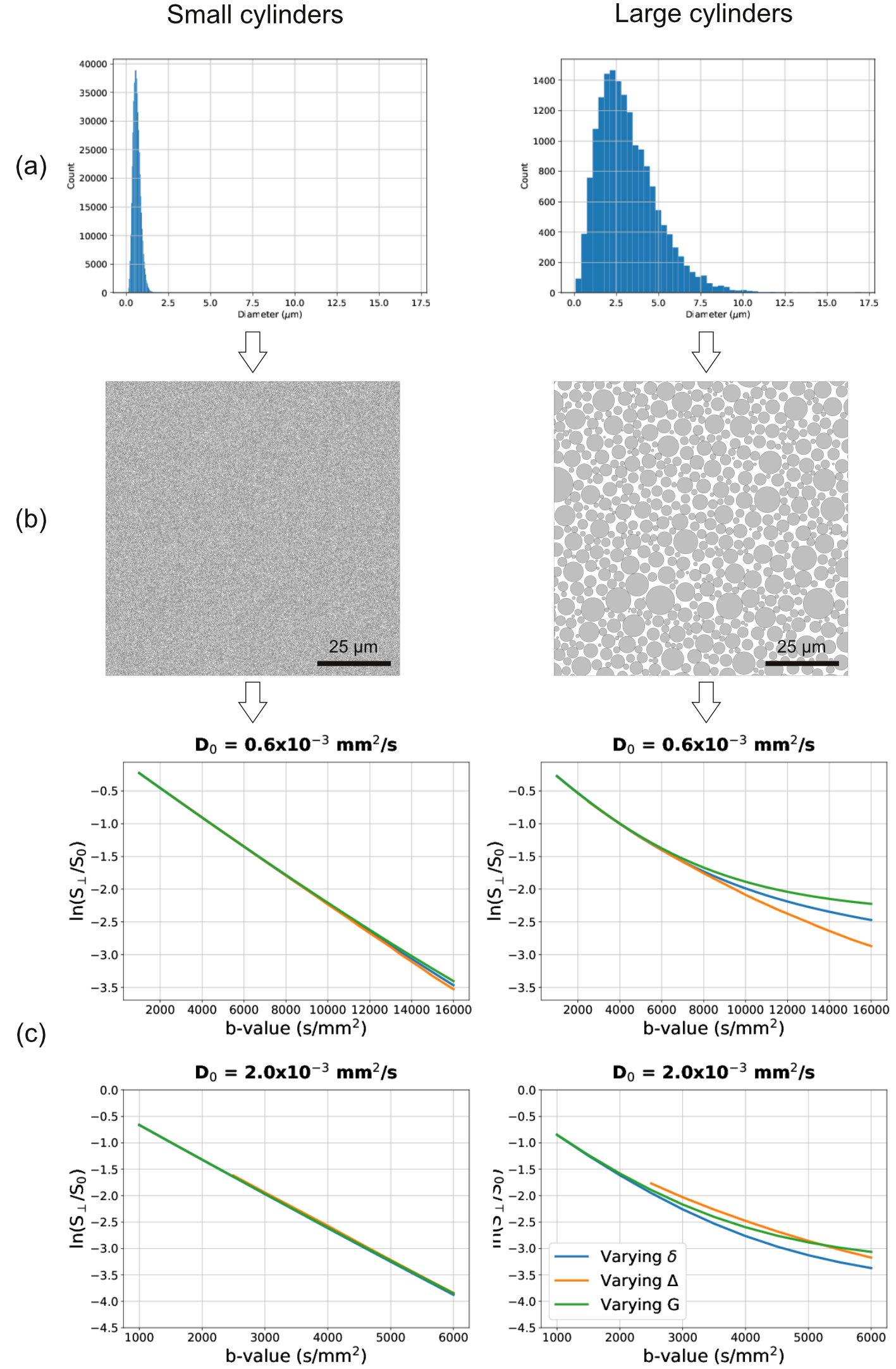
22 gamma distributions from histological studies10,11,12 were used to generate substrates with restricted volume fractions of 50, 60 and 70% (Figure 1). The diffusion signal was generated using the MC/DC Monte Carlo simulator13 (1M spins in the extra-axonal space, voxel size of 0.5x0.5x0.5mm3, periodic cylinder positions14). Experiments mimicking ex-vivo ($$$D_0$$$=0.6x10⁻³mm2/s) and in-vivo ($$$D_0$$$=2.0x10⁻³mm2/s) conditions were conducted. Protocols included a selection of b-values with varying either G, $$$\Delta$$$ or $$$\delta$$$ while keeping the other two parameters constant (Table 1). One b-value could therefore have up to 3 different signal values depending on the choice of G, $$$\Delta$$$ or $$$\delta$$$. Samples were acquired in 60 directions homogeneously covering the unit sphere. Signals were contaminated with rician noise (SNR=30 for ex-vivo and SNR=60 for in-vivo, as most in-vivo non-perpendicular samples were below the SNR=30 floor). The HOTmix dictionary was built by discretizing $$$D_\perp^{(2)}$$$ and $$$\sqrt{D_\perp^{(4)}}$$$ (5 values between [1x10-6,0.4x10-3]mm2/s and 5 values between [0,1.414x10-5]mm2/$$$\sqrt{s}$$$ for ex-vivo, and [1x10⁻⁴, 2x10⁻³]mm2/s and [1x10-5,5x10-5]mm2/$$$\sqrt{s}$$$ for in-vivo conditions, respectively). Cylinder orientation and $$$D_\parallel^{(2)}$$$ were estimated by fitting a DT to the b-values lower than 2’000s/mm2. The HOTmix model was compared to the DT, KT and a single HOT tensor. For a fair comparison, only the perpendicular components were estimated, after factoring out the effect of the orientation and $$$D_\parallel^{(n)}$$$ estimated previously. Estimated parameters were used to reconstruct the signal for a protocol with perpendicular samples only, and with a higher sampling of b-values (each 500 s/mm2). Each model was evaluated by computing the Relative Mean Absolute Error (RMAE) between the reconstructed signal $$$\hat{S}$$$ and the noiseless signal $$$S$$$ simulated using the perpendicular protocol:$$$\frac{\sum_{i=1}^N\frac{|\hat{S_i}-S_i|}{|S_i|}}{N}$$$.Results and discussion
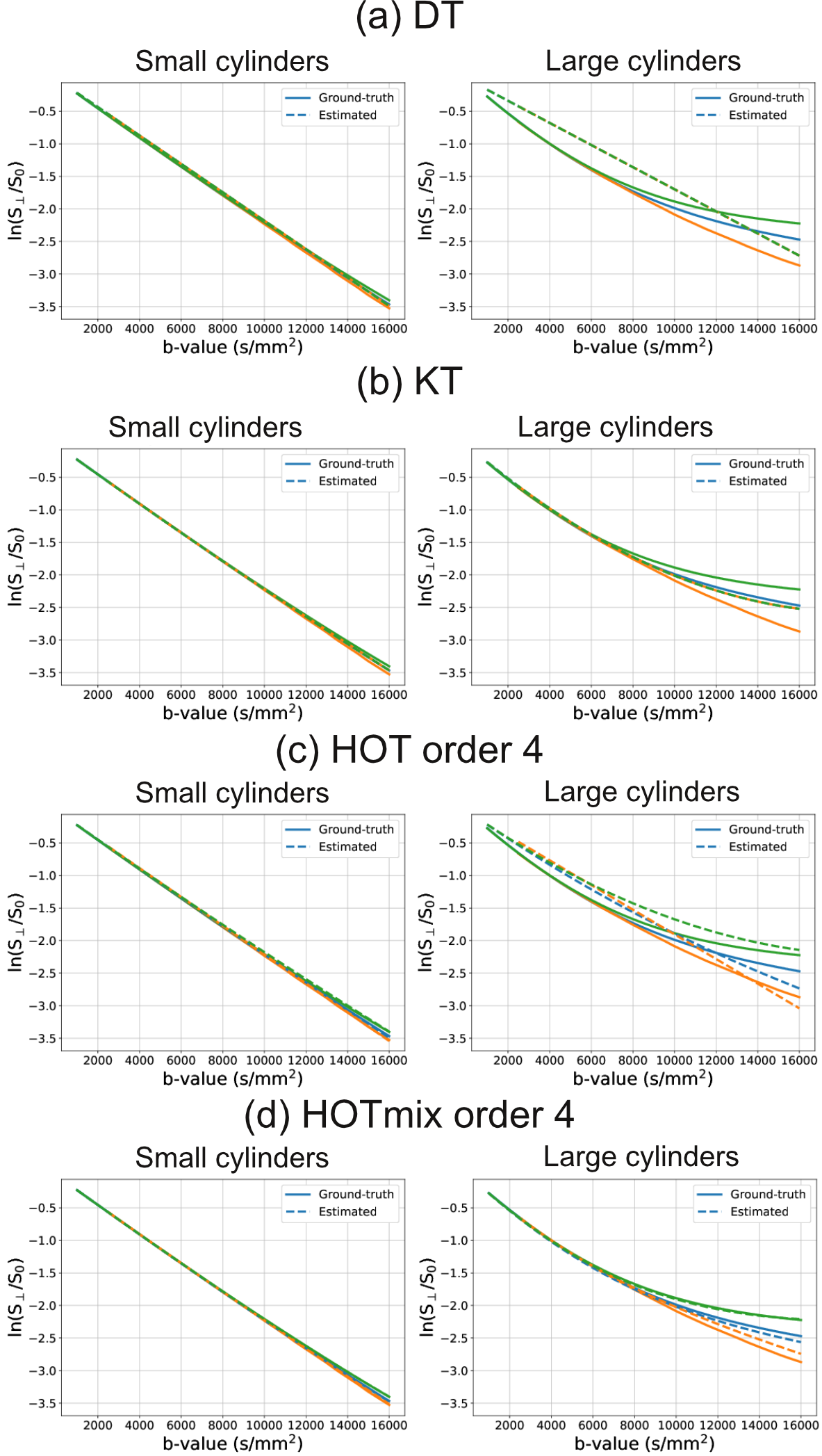
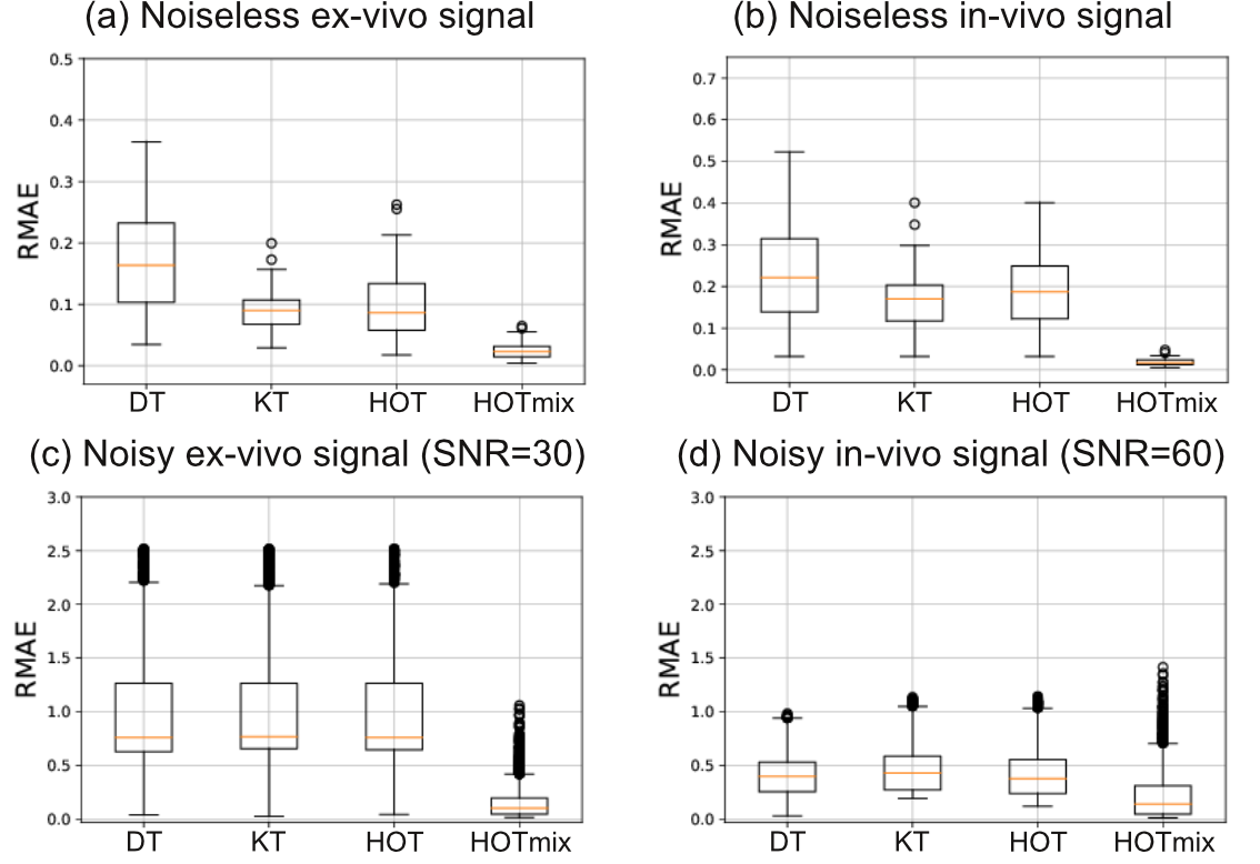
Figure 2 shows the reconstructed signal and the ground truth for the ex-vivo experiments (fitting the noiseless signal). The DT model was unable to capture neither the curvature nor the different offsets of the curves. The DK model captured the curvature but not the different offsets. The HOT model distinguished the 3 curves but was unable to capture the correct curvature. Finally, HOTmix was able to reconstruct the noiseless signal accurately. Results were similar for the in-vivo experiments (not shown). Figure 3 summarizes the RMAE distribution over all substrates and experiments. HOTmix had the lowest mean RMAE and was the only model able to disentangle accurately the effects of the different sequence parameters, in particular $$$\Delta$$$ and $$$\delta$$$, owing to the explicit dependence of the 2nd-order terms on the timing parameters of the diffusion sequence.Conclusion
HOTmix yields better reconstructions of the hindered dMRI signal at intermediate diffusion times compared to the DT, KT and HOT models, adapting to both ex-vivo and in-vivo conditions. A better description of the signal is likely to improve estimates of microstructural features.4 The estimated parameters might also provide information on the substrate microstructure, like hindered volume fraction or outer axon mean diameter. In future work, we will explore whether using HOTmix improves microstructural features estimated from dMRI.Acknowledgements
This work was funded by the Swiss National Science Foundation (SNSF). Marco Pizzolato is supported by the Swiss National Science Foundation under grantnumber CRSII5_170873 (Sinergia project)References
1. Assaf Y, Blumenfeld‐Katzir T, Yovel Y, Basser PJ. AxCaliber: a method for measuring axon diameter distribution from diffusion MRI. Magn Reson Med. 2008;59:1347-1354.
2. Alexander DC, Hubbard PL, Hall MG, et al. Orientationally invariant indices of axon diameter and density from diffusion MRI. Neuroimage. 2010;52(4):1374-1389.
3. Zhang H, Schneider T, Wheeler-Kingshott CA, Alexander DC. NODDI: practical in vivo neurite orientation dispersion and density imaging of the human brain. Neuroimage. 2012;61(4):1000-1016.
4. De Santis S, Jones DK, Roebroeck A. Including diffusion time dependence in the extra-axonal space improves in vivo estimates of axonal diameter and density in human white matter. Neuroimage. 2016;130:91-103.
5. Dyrby T, Sogaard L, Hall M, Ptito M, Alexander DC. Contrast and stability of the axon diameter index from microstructure imaging with diffusion MRI. Magn Reson Med. 2013;70:711-721.
6. Liu C, Bammer R, Acar B, Moseley ME. Characterizing non-gaussian diffusion by using generalized diffusion tensors. Magn Reson Med. 2004;51(5):924-937.
7. Daducci A, Canales-Rodríguez EJ, Zhang H, Dyrby TB, Alexander DC, Thiran J-P. Accelerated Microstructure Imaging via Convex Optimization (AMICO) from diffusion MRI data. Neuroimage. 2015;105:32-44.
8. Yablonskiy DA, Bretthorst GL, Ackerman JJH. Statistical model for diffusion attenuated MR signal. Magn Reson Med. 2003;50(4):664-669.
9. Novikov DS, Fieremans E., Jespersen SN, Kiselev VG. Quantifying brain microstructure with diffusion MRI: Theory and parameter estimation. NMR in Biomedicine. October 2018.
10. Lamantia A-S, Rakic P. Cytological and quantitative characteristics of four cerebral commissures in the rhesus monkey. J Comp Neurol. 1990;291(4):520-537.
11. Aboitiz F, Scheibel AB, Fisher RS, Zaidel E. Fiber composition of the human corpus callosum. Brain Res. 1992;598(1-2):143-153.
12. Alexander DC, Hubbard PL, Hall MG, et al. Orientationally invariant indices of axon diameter and density from diffusion MRI. Neuroimage. 2010;52(4):1374-1389.
13. Rafael-Patino J, Girard G, Romascano D et al. Realistic 3D Fiber Crossing Phantom Models for Monte Carlo Diffusion Simulations. Proc. Intl. Soc. Mag. Reson. Med. 26 (2018): 3220.
14. Hall MG, Alexander DC. Convergence and Parameter Choice for Monte-Carlo Simulations of Diffusion MRI. IEEE Trans Med Imaging. 2009;28(9):1354-1364.
Figures