3517
Time-efficient high resolution diffusion weighted SSFP measurements at 14.1T1High-Field Magnetic Resonance Center, Max Planck Institute for Biological Cybernetics, Tübingen, Germany, 2Biomedical Magnetic Resonance, University Hospital Tübingen, Tübingen, Germany, 3Institute for clinical anatomy and cellanalysis, Department of Anatomy, University Hospital Tübingen, Tübingen, Germany
Synopsis
This study investigates the use of diffusion weighted SSFP imaging for high-resolution diffusivity measurements of post-mortem tissue, using two different models (Wu-Buxton and Freed) and draws a comparison to conventional DW SE-Measurements. A toolbox was developed to optimize SSFP imaging parameters for selected tissue regions which was then used successfully. We showed that the SSFP approach is highly valuable for time-efficient high-resolution post-mortem diffusion weighted imaging.
Introduction
Stejskal-Tanner based diffusion weighted imaging (EPI) sequences require long measurement times to achieve a high diffusion to noise ratio. Due to potential advantages in speed, SSFP has proven useful for high-resolution post-mortem applications. For modeling the diffusion weighted SSFP signal the Wu-Buxton1 and the Freed model2 can be used. This study verifies their use for high-resolution DW SSFP imaging in post-mortem human brain tissue. Specifically it evaluates the impact of: flip angle, T1 and T2-relaxation, signal-to-noise-ratio (SNR) and diffusion-contrast-to-noise levels on mean diffusivity maps.
A
method was developed to optimize
SSFP sequence parameters, with the aim to improve SNR in
regions of interest (ROI) such as cortical gray matter or white
matter fibers.
Materials and Methods
Data recording
Human post-mortem brain samples ( 81y female, 80y male, from the body-donor programme of the University of Tübingen) of approx. 4×2×2.5 cm were dissected from the occipital region, so to include the calcarine sulcus. The samples were placed in a cylindrical sample holder and submerged in Fomblin (Solvay Solexis inc., Italy).
All measurements were performed on a 14.1T MRI scanner (Bruker Biospec, Ettlingen, Germany) and included flip angle mapping, T1 and T2 mapping. A diffusion weighted SSFP sequence (McNab and Miller3) was used to record multiple DW SSFP data sets. As a gold-standard for diffusion coefficients, a diffusion weighted 3D-spin echo EPI sequence was run. A self written MATLAB package for simulation and image analysis supports both the Wu-Buxton model and the Freed model for SSFP data analysis.
Measurement parameters were as follows: AFI: TR=20/100ms, FA=60deg, TE=4ms, voxel size: 0.93mm isotropic. T1: MPRAGE, TI=10/50/100/250/500/1000/2000/3000ms, TR=4300, FA=8deg, TE=2ms, voxel size: 0.3mm isotropic. T2: Multi-spin-echo, TR= 4000s, TE=6:6:90ms, voxel size:0.3x0.3x1mm. SSFP: TE=3.97ms, FA=17deg, τ=1.11ms/1.85ms/2.85ms/4.30ms, G=100/200/300/400 mT/m, voxel size=0.3mm isotropic, 64 directions, TR=τ+3.85ms. EPI: TE=19ms, TR=500ms, FA=70deg, b=5000s/mm2, 64 directions
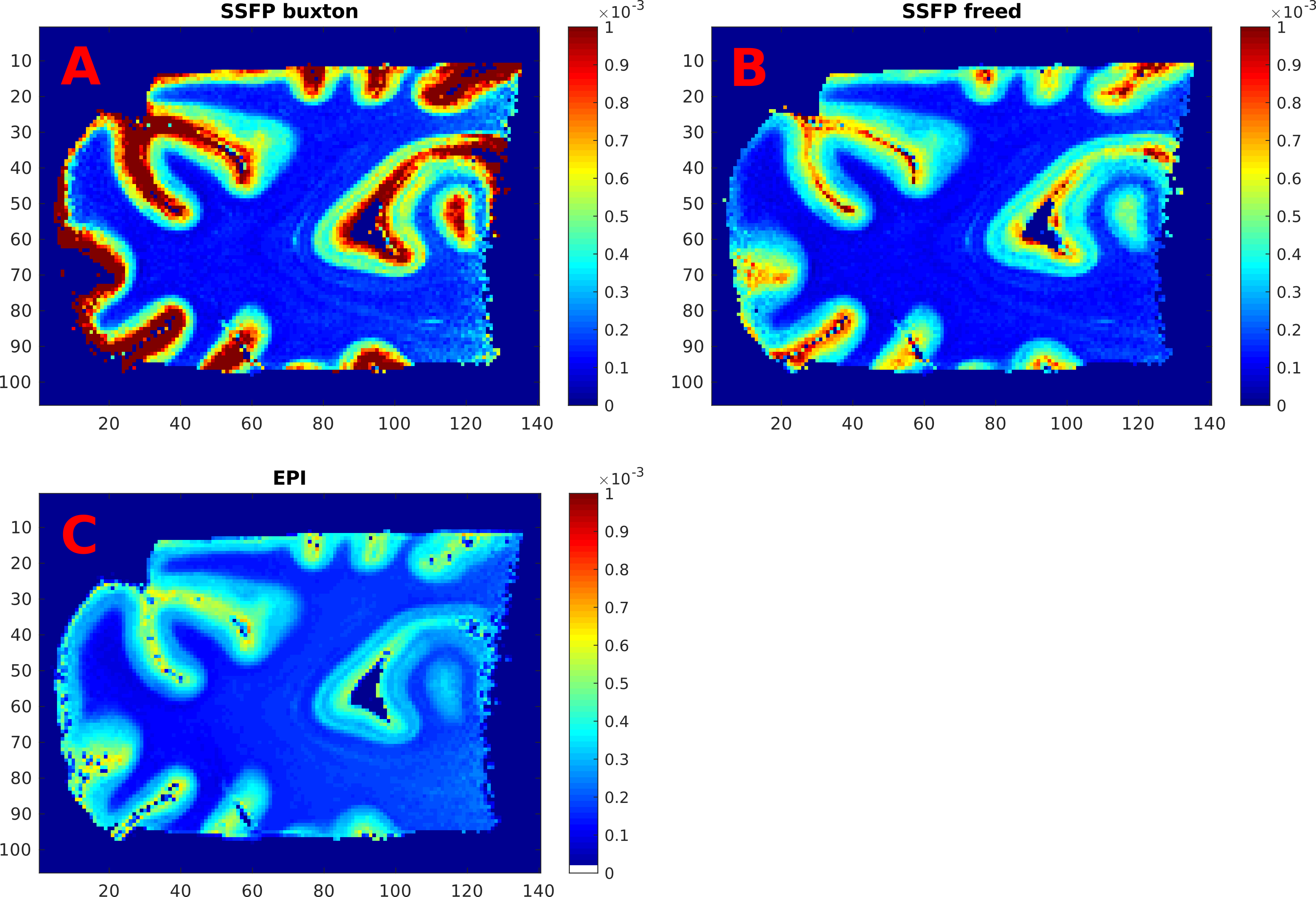
Buxton vs Freed vs EPI
Apparent diffusion coefficients (ADC) were reconstructed and mean diffusivity (MD) maps were calculated. Both the Wu-Buxton model and the Freed model were used to reconstruct diffusion coefficients from the measured SSFP datasets, using average T1 and T2 values. Likewise MD maps were generated for the Stejskal-Tanner measurements (3D-SE-EPI).
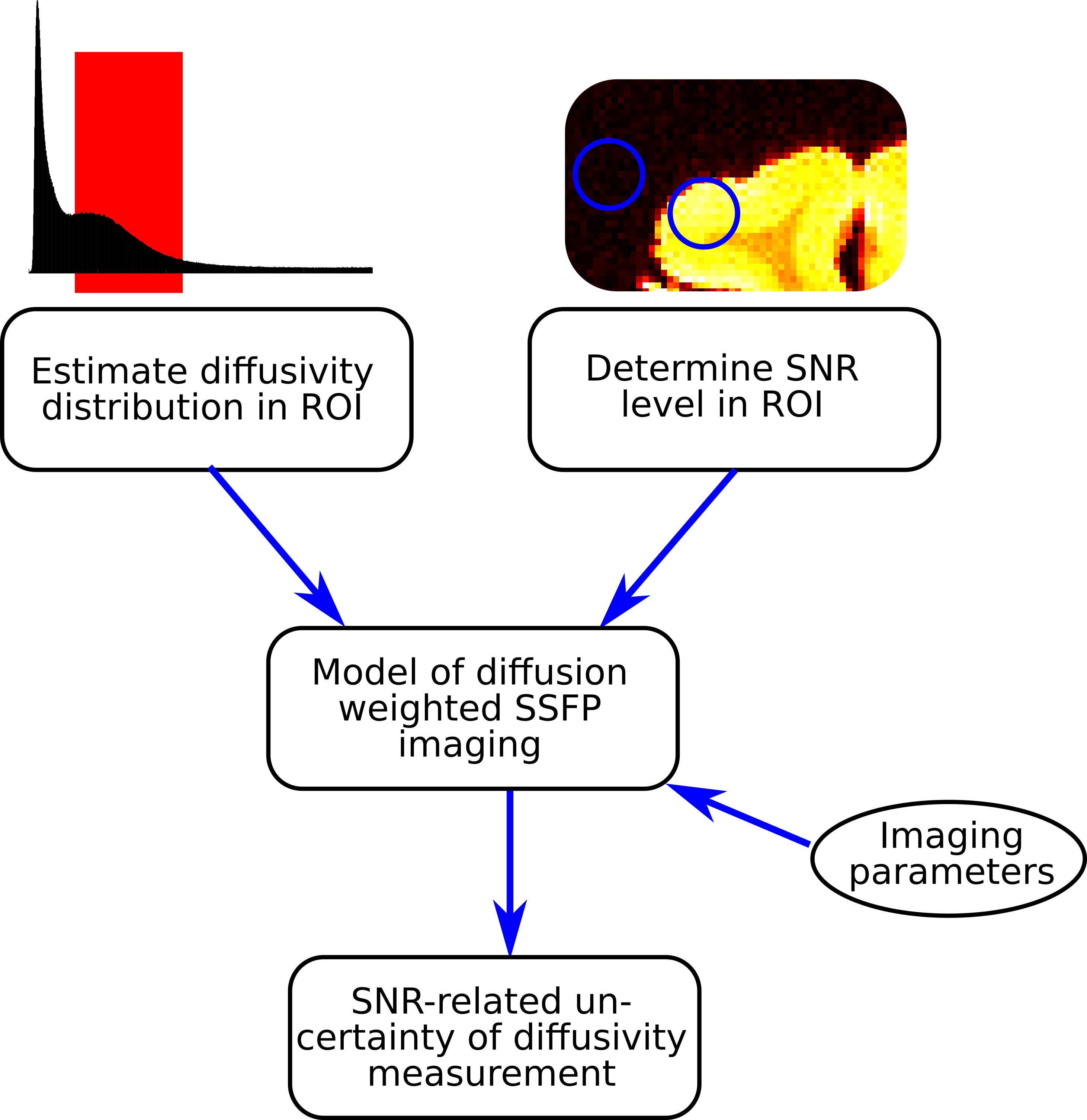
Finding optimized SSFP sequence parameters for selected ROI
The ADC and SNR inside a region of interest were measured from the SSFP datasets. The SNR and diffusivity distribution were then propagated through the Wu-Buxton model in order to calculate the measurement uncertainty of the ADC which is caused by signal noise (Fig.1). SSFP sequence parameters were optimized to minimize the ADC measurement uncertainty in the ROI. Subsequently, the usefulness of those parameters was verified using a new sample.
Results and Discussion
In simulations we found that the relevant T1 (range 500-700ms, average 629ms) and T2 times (range 15-17ms, average 15.6ms) only had a minor influence on the SSFP results. At representative diffusivities of 0.17 and 0.4 mm²/sec, the maximum ΔADC due to T2 inhomogeneities was 2.3% resp. 2.5%, while the maximum ΔADC due to T1 inhomogeneities was 6.9% resp. 6.7%. Therefore time-consuming high resolution T1 and T2 measurements could be omitted in further measurements and a rough estimate was considered sufficient. The flip angle dependency, on the other hand, was high, so flip angle maps were always recorded.
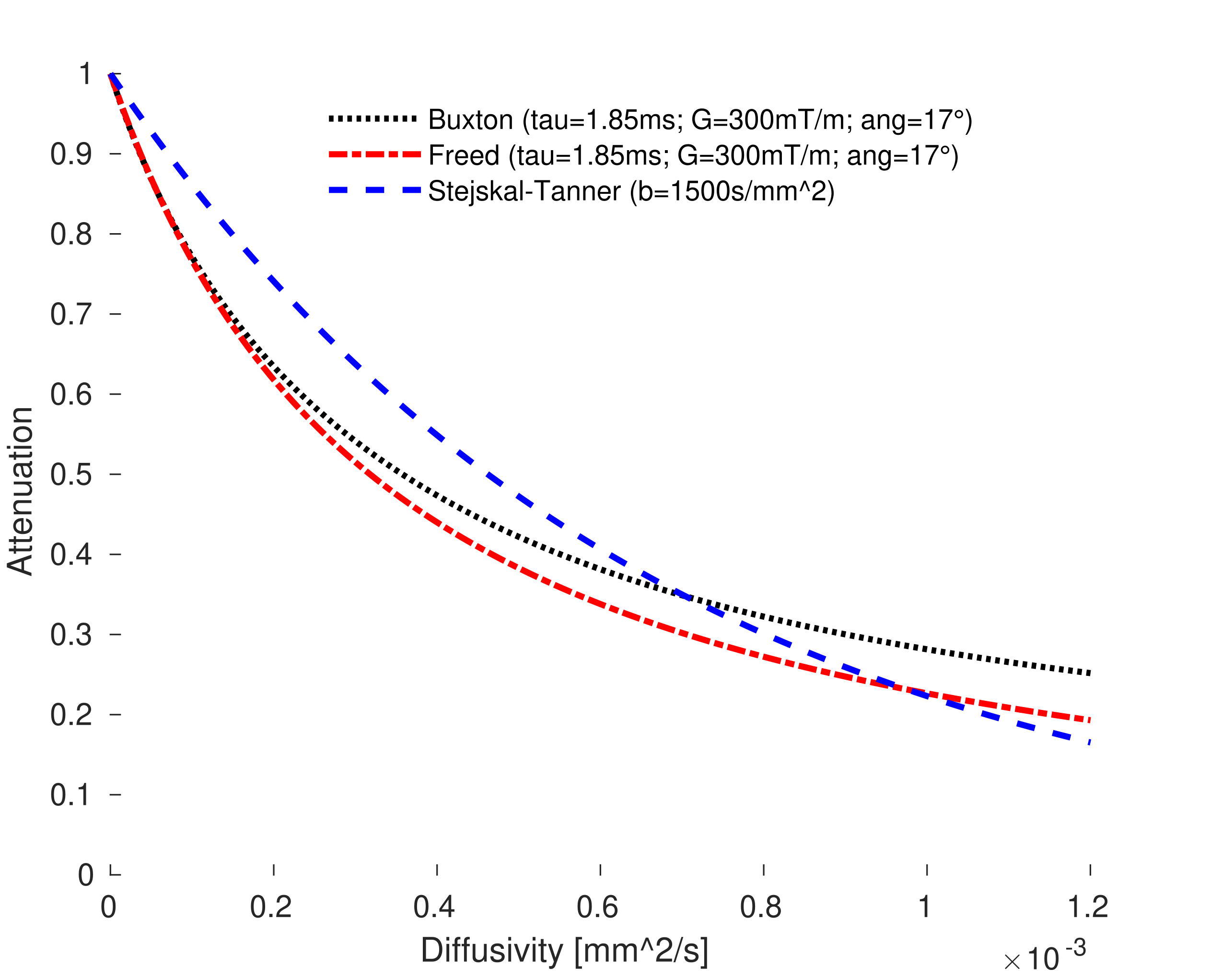
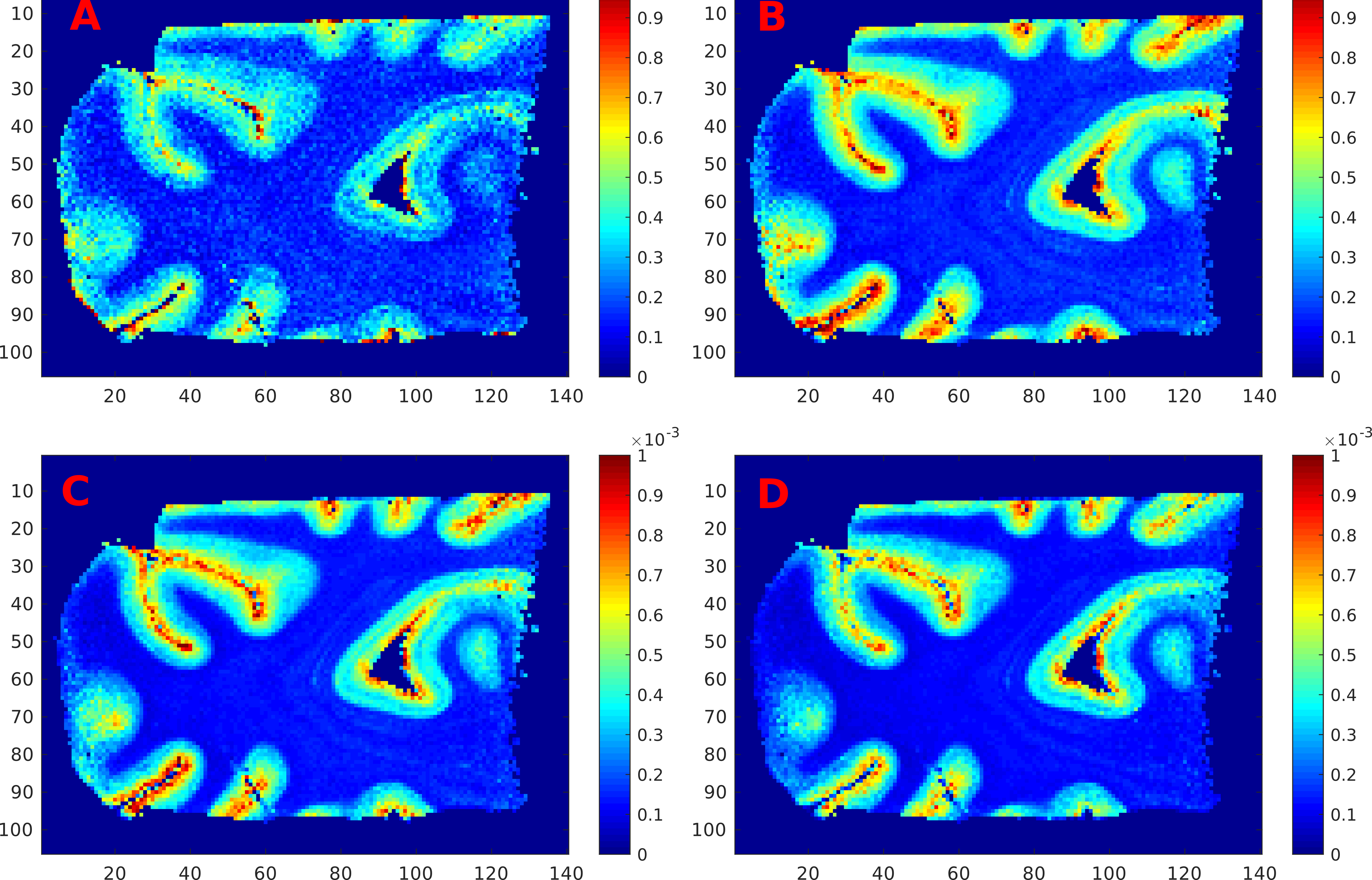
Simulations showed (Fig.2) that the dynamic range in both SSFP models is better for areas with low diffusivity while the Stejskal-Tanner model yields a more homogeneous weighting. Optimal sequence parameters were predetermined in order to optimize SNR in white matter. (Results see Fig.5). Even though a good correspondence between the methods is found in the white matter, the deviations in cortical areas are significant.
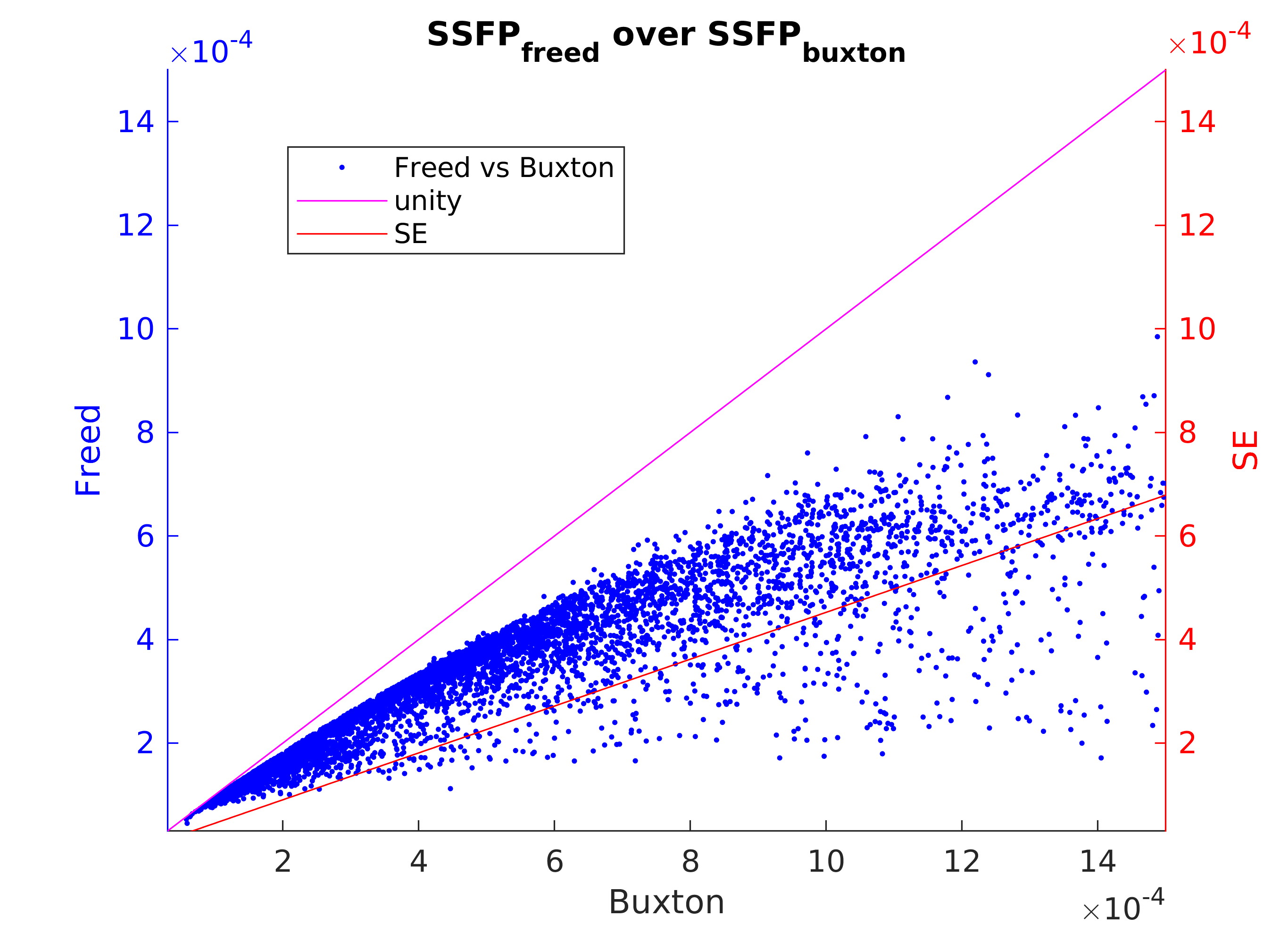
We found that the Freed-model gave SSFP results that more closely matched the Stejskal-Tanner method (our gold standard), than the Buxton-model, in agreement with Bieri et al4. Nevertheless, improvements in modeling are needed, since the observed diffusivity in gray matter still significantly deviated from expected values (Fig.3,Fig.4).
The usability of diffusion weighted SSFP data highly depends on the diffusion weighting. While a strong diffusion weighting improves contrast between diffusion weighted and unweighted images especially in low-diffusivity regions, a too strong diffusion weighting reduces the SNR in high-diffusivity areas below an acceptable level. (Fig.5).
We observed that, for the rather large FOV required to image human post-mortem tissue, Stejskal-Tanner measurements with voxel sizes below 300µm were sub-optimal in terms of the available SNR per time, likely due to long TE times. On the contrary with SSFP, we could perform high quality tensor diffusion imaging with 4 averages, a FOV of 36.1×24.8×24.8mm and a voxel size of 172µm, in only 16h.
Conclusion
The SSFP approach offers time-efficient high-resolution post-mortem diffusion weighted imaging, provided that accurate modelling and optimized sequence parameters are used.Acknowledgements
No acknowledgement found.References
1. Buxton, Richard B. "The diffusion sensitivity of fast steady‐state free precession imaging." Magnetic resonance in medicine 29.2 (1993): 235-243.
2. Freed, D. E., et al. "Steady-state free precession experiments and exact treatment of diffusion in a uniform gradient." The Journal of Chemical Physics 115.9 (2001): 4249-4258.
3. McNab, Jennifer A., and Karla L. Miller. "Steady‐state diffusion‐weighted imaging: theory, acquisition and analysis." NMR in Biomedicine 23.7 (2010): 781-793.
4. Bieri, O., et al. "Fast diffusion‐weighted steady state free precession imaging of in vivo knee cartilage." Magnetic resonance in medicine 67.3 (2012): 691-700.
Figures