3492
Optimized diffusion gradient waveforms for estimating surface-to-volume ratio of an anisotropic medium1Laboratoire PMC, Ecole Polytechnique, Palaiseau, France, 2NORMENT, KG Jebsen Centre for Psychosis Research, Oslo University Hospital, Oslo, Norway, 3Institute of Clinical Medicine, University of Oslo, Oslo, Norway
Synopsis
We present here a simple and efficient algorithm for designing of diffusion gradient profiles allowing one to implement prescribed theoretical properties. This algorithm generalizes the well-known sine and cosine decomposition and can handle various experimental constraints. Relying on recent diffusion MRI theoretical advances, we apply it to the challenging problem of estimating the surface-to-volume ratios in anisotropic media.
Introduction
Since the seminal paper by Mitra et al.1, diffusion NMR has been widely used to estimate the surface-to-volume ratio of a sample and related typical sizes of compartments and pores. Recent advances in diffusion MRI such as double diffusion encoding2 and isotropic diffusion encoding schemes3 potentially extend the applicability of complex diffusion MR approaches to human MR scanners. In turn, such scanners require careful manipulations with RF and gradient coils/amplifiers in order to avoid possible destruction, breaks or subject injuries. Here we address the challenging problem of precisely estimating the surface-to-volume ratio of an anisotropic medium with 3D gradient sequences. Relying on recent theoretical advances4, we propose a simple and robust algorithm for designing optimized gradient profiles with prescribed properties that incorporate most practical constraints for human MR imaging.Methods
We consider a spin-echo experiment with an applied diffusion encoding gradient $$$\boldsymbol{g}(t)$$$ from $$$t=0$$$ to the echo time $$$t=T$$$. The main idea of the algorithm is to choose a family of functions $$$\left(f_1(t),\ldots, f_k(t)\right)$$$ (for example, (co)sines, polynomials, ...) and write the three-dimensional gradient $$$\boldsymbol{g}(t)$$$ as a linear combination of these basis functions
$$\begin{pmatrix}g_x(t)\\g_y(t)\\g_z(t)\end{pmatrix}=\mathcal{X}\begin{pmatrix}f_1(t)\\\vdots\\f_k(t)\end{pmatrix}\;,$$
where $$$\mathcal{X}$$$ is the $$$3\times k$$$ weights matrix that we seek to optimize. This is a generalization of the classical sine and cosine decompositions. Some constraints on the gradient profile may be satisfied by a suitable choice of the basis functions $$$\left(f_1(t),\ldots, f_k(t)\right)$$$. For example, one can ensure the smoothness of the gradient profile by choosing a family of smooth
functions such as polynomials. In the same way, the refocusing
condition $$$\int_0^T \boldsymbol{g}(t)\,\mathrm{d}t=\boldsymbol{0}$$$ can be achieved by choosing zero-mean functions, for example, (co)sines with an integer number of periods. It is also possible to add
some constraints as a part of the optimization process (see below some
examples).
It was recently derived in Ref4 that one can estimate the
surface-to-volume ratio of an anisotropic medium by using gradient sequences
that satisfy a particular ``isotropy’’ matrix condition, $$$\mathcal{F}^{(3)}\propto I$$$, where
$$\mathcal{F}^{(m)}=-\frac{\gamma^2}{2}\int_0^T\int_0^T\boldsymbol{g}(t_1)\boldsymbol{g}(t_2)\lvert t_2 - t_1 \rvert^{m/2} \,\mathrm{d}t_1 \,\mathrm{d}t_2$$
(with $$$m=3$$$), and $$$I$$$ is the $$$3\times 3$$$ unit matrix. We used the tensor product notation: if $$$\boldsymbol{a}$$$ and $$$\boldsymbol{b}$$$ are vectors, then $$$\boldsymbol{a}\otimes\boldsymbol{b}$$$ is a matrix with components $$$\left(\boldsymbol{a}\otimes\boldsymbol{b}\right)_{ij}=a_ib_j$$$. Note that original isotropic diffusion weighting sequences3 satisfy a
different condition, namely $$$\mathcal{F}^{(2)}\propto I$$$ (one can indeed show that $$$\mathcal{F}^{(2)}$$$ is actually the $$$b$$$-matrix, with $$$\mathrm{Tr}\left(\mathcal{F}^{(2)}\right)=b$$$. We thus search for a 3D gradient profile $$$\boldsymbol{g}(t)$$$ that makes the $$$\mathcal{F}^{(3)}$$$ matrix ``isotropic''. Moreover, one can incorporate other constraints such as vanishing $$$\mathcal{F}^{(4)}$$$ matrix for a more accurate estimation of the surface-to-volume ratio.
From a numerical point of view, the computation of the $$$\mathcal{F}^{(m)}$$$ matrices involves a tradeoff between precision and speed. Improving the speed of
computations is especially important in the context of optimization algorithms,
which usually require numerous iterations. By pre-computing the $$$k\times k$$$ matrices $$$\mathcal{A}^{(m)}$$$:
$$\mathcal{A}^{(m)}_{i,j}=-\frac{\gamma^2}{2}\int_0^T\int_0^T f_i(t_1)f_j(t_2)\lvert
t_2 - t_1 \rvert^{m/2} we \,\mathrm{d}t_1 \,\mathrm{d}t_2\;,$$
we can compute the $$$\mathcal{F}^{(m)}$$$ matrices directly from $$$\mathcal{X}$$$ by $$$\mathcal{F}^{(m)}=\mathcal{X}\mathcal{A}^{(m)}\mathcal{X}{}^T$$$. The initial computation of the $$$\mathcal{A}^{(m)}$$$ matrices is the most time-consuming step but it has to be done only
once. The consequent computations of $$$\mathcal{F}^{(m)}$$$ involve just matrix multiplications whose size is given by the size of
the family $$$\left(f_1(t),\ldots,f_k(t)\right)$$$, independent of the numerical sampling of the time interval $$$[0,T]$$$
that controls the accuracy of the computations. A
similar matrix representation is applicable to any linear or bilinear form of
the gradient profile. Common examples include: imposing zeros of the gradient;
flow-compensation or motion artifact suppression conditions; controlling heat
generation of the sequence; computing the $$$b$$$-value.
Results
Figure 1 shows an example of a gradient sequence, which was generated by our algorithm from $$$9$$$ piecewise polynomials of order $$$5$$$. We imposed the conditions $$$\boldsymbol{g}(0)=\boldsymbol{g}(T/2)=\boldsymbol{g}(T)=\boldsymbol{0}$$$ as well as $$$\mathcal{F}^{(3)}\propto I$$$ and $$$\mathcal{F}^{(4)}=0$$$.The decomposition over a relatively small set of functions is not complete, hence the algorithm returns optimized solutions that are not ``optimal’’ in the common sense. One may improve the result returned by the algorithm by adding more functions into the family. Moreover, this would increase the dimensionality of the functional space spanned by $$$\left(f_1(t), \ldots, f_k(t)\right)$$$, which usually leads to many possible gradient sequences that satisfy the chosen constraints. This property can be advantageous in practice, as one can design many optimized solutions.
Conclusion
In conclusion, the proposed algorithm is simple, computationally efficient, flexible, and is able to handle various constraints, such as motion artifacts of eddy-current distortions, which makes it an excellent tool for further development and design of complex diffusion encoding schemes. In particular, accurate surface-to-volume ratios in anisotropic media may help to introduce new biomarkers and to investigate mesoscopic anisotropy of biological samples, for example of grey and white matter in the human brain.Acknowledgements
No acknowledgement found.References
[1] P. P. Mitra, P. N. Sen, L. M. Schwartz, and P. Le Doussal, Phys. Rev. Lett. 68 3555-3558 (1992)[2] Yang et al., MRM 80 507 (2018)
[3] S. Eriksson, S. Lasič, and D. Topgaard, J. Magn. Res. 226 13-18 (2013)
[4] N. Moutal, I. I. Maximov, and D. S. Grebenkov, ArXiv: 1811.01568
Figures
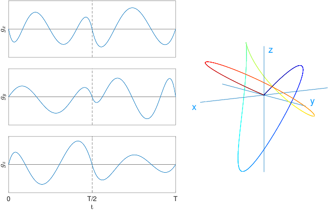
(left) Graphs of the three spatial components of the gradient $$$\boldsymbol{g}(t)$$$. (right) Three-dimensional plot of $$$\boldsymbol{q}(t)=\int_0^t \gamma\boldsymbol{g}(t')\,\mathrm{d}t'$$$. the color encoding of the trajectory represents time, from $$$t=0$$$ (blue) to $$$t=T$$$ (red).