3490
The tuned trinity of b-tensors1Random Walk Imaging, Lund, Sweden, 2Danish Research Centre for Magnetic Resonance, Centre for Functional and Diagnostic Imaging and Research, Copenhagen University Hospital Hvidovre, Copenhagen, Denmark, 3Division of Physical Chemistry, Department of Chemistry, Lund University, Lund, Sweden, Lund, Sweden
Synopsis
Unprecedented microstructural details of heterogeneous materials such as tissue are non-invasively accessible by multidimensional diffusion encoding (MDE) MRI using varying shapes of b-tensors. MDE can probe multidimensional distributions of diffusion tensors in terms of their size, shape and orientation. For robust conclusions, time-dependent diffusion effects need to be considered in MDE. A convenient recipe for generating b-tensors of varying shape was implemented including a single adjustable tuning parameter. The resulting b-tensors can thus be tuned for sensitivity to time-dependent diffusion.
Introduction
Microstructural features of heterogeneous materials, such as average cell eccentricity or variance of cell density, which are inferred from optical microscopy images, can be quantified non-invasively by multidimensional diffusion encoding (MDE) MRI using varying shapes of b-tensors1-5. With MDE, distributions of diffusion tensors can be characterized in terms of size, shape and orientation3,4. This information is directly encoded in the measured signal by MDE, which is not possible by conventional diffusion MRI. In contrast, due to the inability of providing more specific data, conventional approaches heavily rely on data modeling assumptions, rendering conclusions unreliable6,7. If not accounted for, time-dependent diffusion effects may still skew MDE results. This can happen if different b-tensors are probing diffusion at different time scales. As we have demonstrated previously using spherical and linear b-tenors, spectral analysis of encoding and diffusion allows designing tuned MDE waveforms, which yield equal first-order signal attenuation. The tuning dimension also provides an additional orthogonal measurement suited to probe correlations between anisotropy and size of restrictions8. A convenient recipe can be used to yield b-tensors with arbitrary anisotropy and asymmetry3,4. Here we have implemented spectral tuning by modifying the previous recipe with a single adjustable tuning parameter.
Frequency analysis of encoding
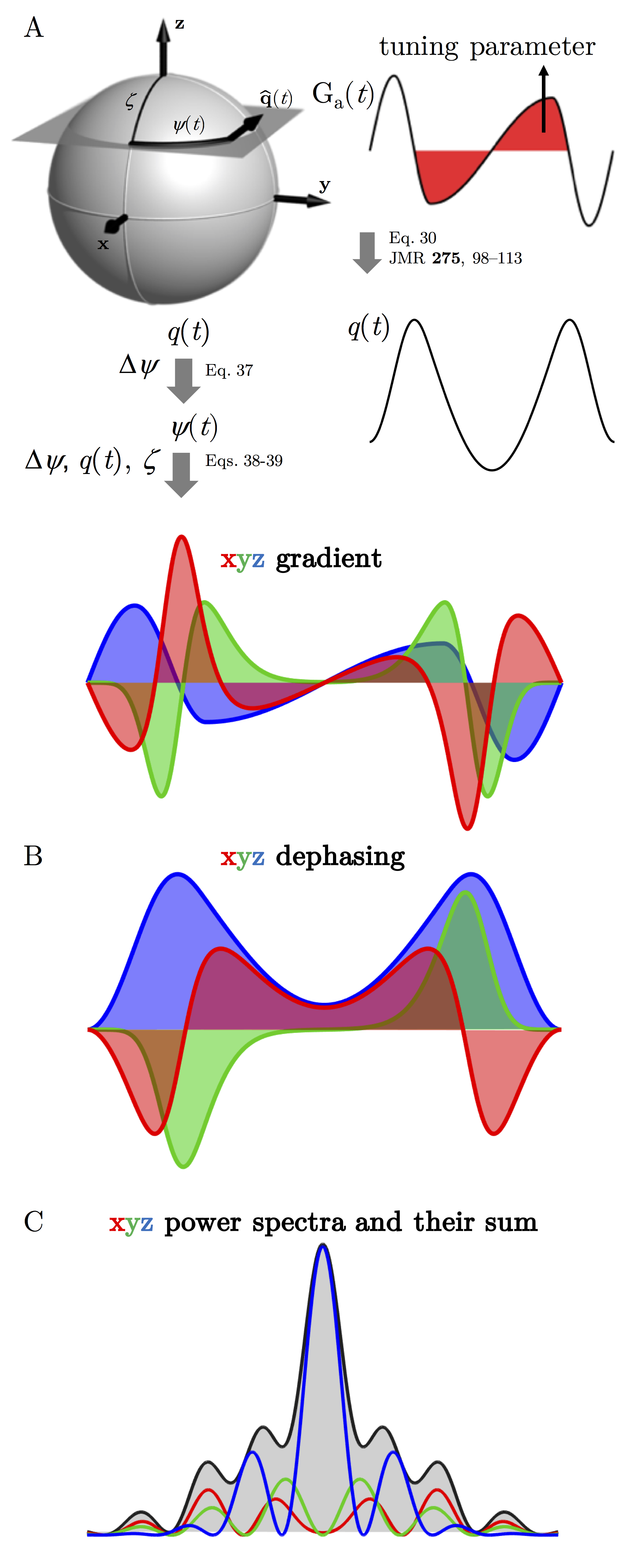
To the first order, signal attenuation is given by9 $$\beta = \frac{1}{2\pi}\int_{-\infty}^{\infty} F_{i}(\omega) D_{ij}(\omega) F^*_{j}(\omega) d\omega,$$ where we adopt the Einstein summation convention, $$$\mathbf{D}(\omega)$$$ is the velocity correlation spectrum, $$$\mathbf{F}(\omega)$$$ is the spectrum of dephasing $$\mathbf{F}(\omega) = \int_{0}^{\tau} \mathbf{q} (t) \exp^{-i\omega t}dt$$ and dephasing is given by the effective gradient as $$$\mathbf{q} (t) = \gamma \int_{0}^{t} \mathbf{G} (s) ds$$$. Directional average of the power spectrum, $$$F_{i}(\omega) F^*_{j}(\omega)$$$, is given by the sum of power spectra along any three orthogonal axes, i.e. by the trace at each frequency. Integration of the power spectrum over the entire frequency range yields the b-tensor, $$b_{ij} = \frac{1}{2\pi}\int_{-\infty}^{\infty} F_{i}(\omega) F^*_{j}(\omega) d\omega$$.Designing tuned b-tensors of varying shape
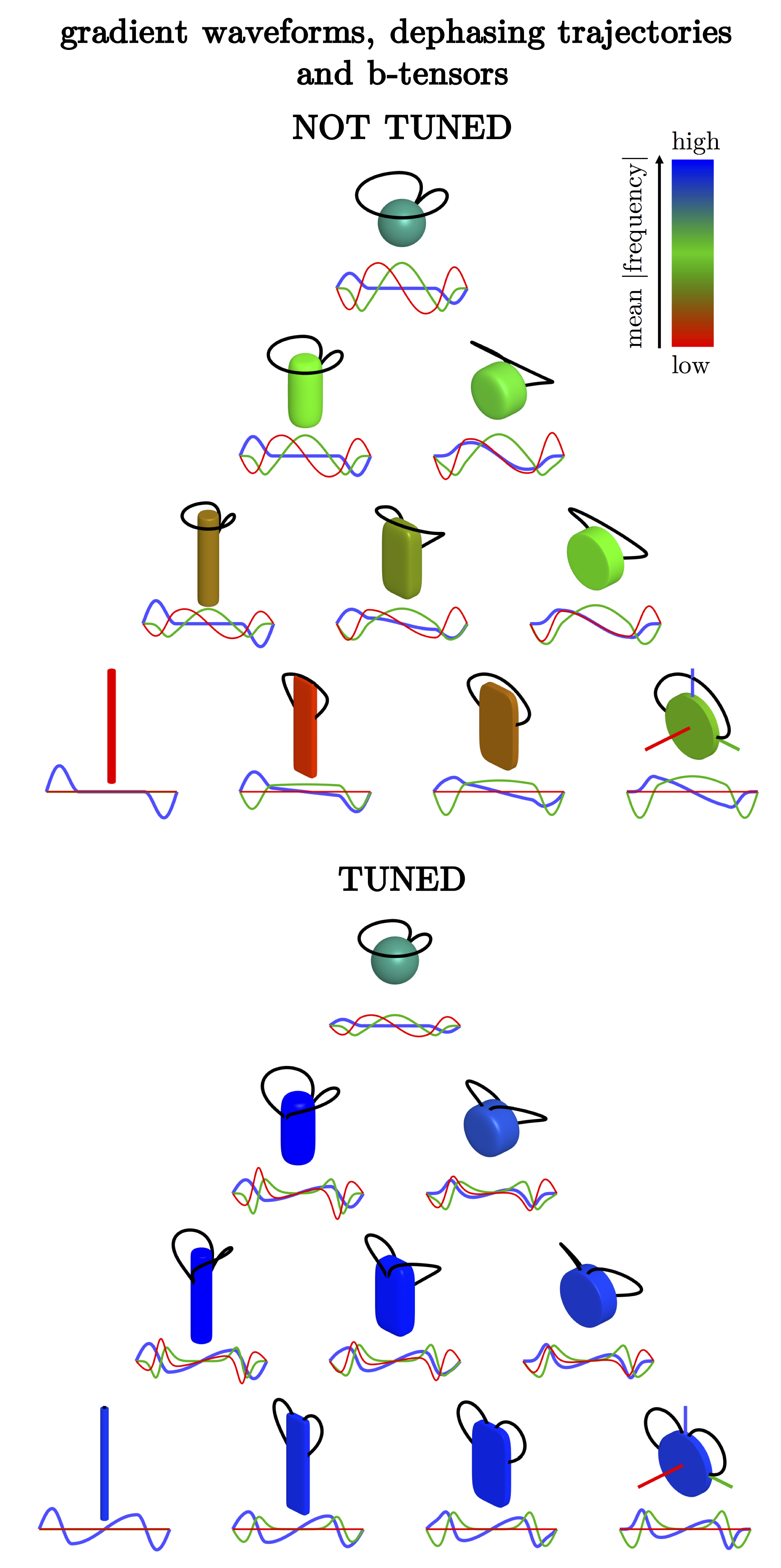
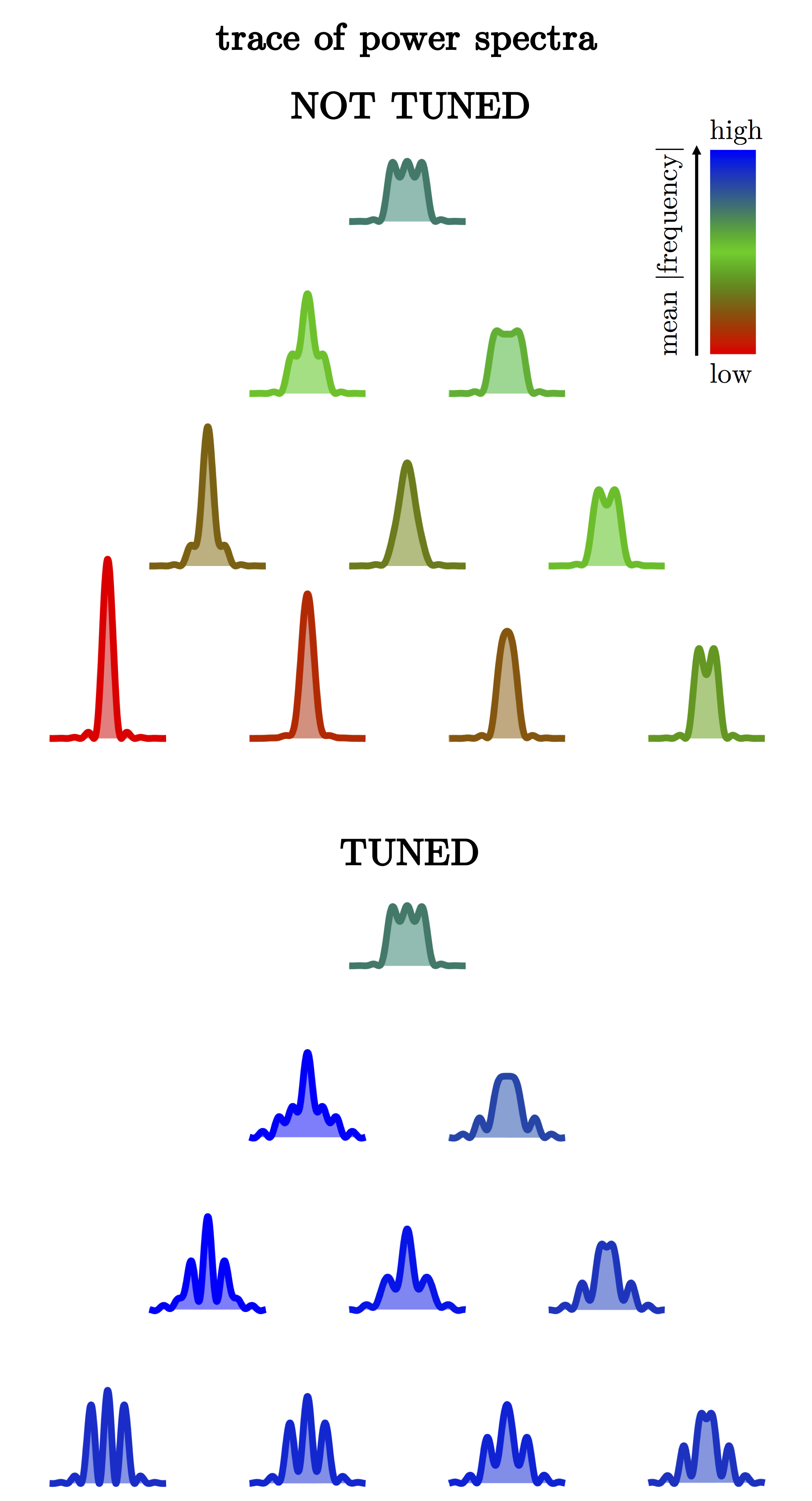
Various b-tensor shapes and the associated q-trajectories can be constructed using two key parameters: $$$\zeta$$$ and $$$\Delta\Psi$$$, yielding anisotropy and asymmetry of b-tensors, $$$\it{b}_{\mathrm{\Delta}}$$$ and $$$\it{b}_{\mathrm{\eta}}$$$, respectively. Varying anisotropy and asymmetry of b-tensors allows detecting anisotropy and asymmetry of diffusion tensors. Gradient waveforms are generated following the steps outlined in refs. 3,4 and illustrated in Fig. 1A. First, the azimuth angle $$$\Psi(t)$$$ is calculated from gradient $$$G_{\mathrm{a}}(t)$$$ and $$$\Delta\Psi$$$. Then, the polar angle $$$\zeta$$$ is used to yield $$$\mathbf{G}(t)$$$ and the corresponding dephasing $$$\mathbf{q}(t)$$$ (Fig 1B). Introducing the tuning parameter (TP) as an amplitude of oscillation inserted between the bipolar lobes of the $$$G_{\mathrm{a}}(t)$$$ (red patch in Fig. 1A) allows tuning the average dephasing power spectrum shown in Fig. 1C. The TP was adjusted for each b-tensor shape to yield approximately equal apparent isotropic diffusivities for diffusion restricted in a sphere of arbitrary size. The colors for b-tensor shapes and average power spectra shown in Figs. 2 and 3 correspond to the average encoding frequency mapped to the range of colors red-green-blue.Results and discussion
The original recipe3,4 to generate b-tensors of varying shapes (Fig. 2A) can be easily modified to achieve spectral tuning (Fig. 2B) using a single adjustable tuning parameter (TP). An optimal TP can be found considering restricted diffusion. For a spherical restriction, tuning yields approximately equal apparent isotropic diffusivities in the entire range of relative encoding times $$$\sqrt{D_0 \tau}/R$$$ (not shown). Fig. 2 demonstrates how a wide range of average encoding frequencies (color-coded in b-tensor shapes) is homogenized by tuning. The average color-coded power spectra can be seen in Fig. 3. A few caveats need be address with our simplistic tuning implementation. First, our tuning was performed for the case of restricted diffusion with its characteristic diffusion spectrum $$$D(\omega)$$$9. Considering a radically different case of e.g. incoherent flow would present a different tuning problem. Achieving perfect tuning for arbitrary $$$D(\omega)$$$ remains a difficult if not impossible task. Second, in our tuning implementation, we ignored the effects caused by spectral anisotropy10. This effect has been first described by de Swiet and Mitra11 for the case of spherical b-tensors. We have suggested the potential of using spectral anisotropy as yet another encoding dimension exclusively sensitive to anisotropic restrictions10. Third, additional tuning parameters would be necessary to further improve the tuning, which is particularly important when probing anisotropic restricted diffusion. This task is a subject future work. Forth, the suggested waveform design is conceptually neat but not optimal in terms of hardware demands. Although our waveforms can be applied on high performance gradient systems1-5, optimizations considering gradient amplitude, slew and coil heating limitations12 will be needed for efficient clinical applications.
Acknowledgements
HL is kindly supported by the European Research Council under the European Union's Horizon 2020 research and innovation program (grant agreement No. 804647 – C-MORPH)
DT is supported by the Swedish Research Council (VR) 2018-03697 and by the Swedish Foundation for Strategic Research (SSF) ITM17-0267
References
1. Lasič S, Szczepankiewicz F, Eriksson S, Nilsson M, Topgaard D, Microanisotropy imaging: quantification of microscopic diffusion anisotropy and orientational order parameter by diffusion MRI with magic-angle spinning of the q-vector, Front. Phys., 2014, 2, (11), 1–14.
2. Eriksson S, Lasič S, Nilsson M, Westin C-F, Topgaard D, NMR diffusion-encoding with axial symmetry and variable anisotropy: Distinguishing between prolate and oblate microscopic diffusion tensors with unknown orientation distribution, J. Chem. Phys., 2015, 142, 104201.
3. Topgaard D, Director orientations in lyotropic liquid crystals : diffusion MRI mapping of the Saupe order tensor, Phys. Chem. Chem. Phys., 2016, 18, 8545–8553.
4. Topgaard D, Multidimensional diffusion MRI, J. Magn. Reson., 2017, 275, 98–113.
5. Topgaard D, NMR methods for studying microscopic diffusion anisotropy, in Diffusion NMR of confined systems: fluid transport in porous solids and heterogeneous materials, New Developments in NMR no. 9, R. Valiullin, Ed. Cambridge, UK: Royal Society of Chemistry, 2017.
6. Jones DK, Knösche TR, Turner R, White matter integrity, fiber count, and other fallacies: the do’s and don’ts of diffusion MRI, Neuroimage, 2013, 73, 239–254.
7. Novikov DS, Kiselev VG, Jespersen SN, On modeling, Magn. Reson. Med., 2018, 79, 3172–3193.
8. Lundell H, Nilsson M, Dyrby T, Parker G, Cristinacce P, Zhou F, Topgaard D, Lasič S, Microscopic anisotropy with spectrally modulated q-space trajectory encoding., in Proc. Intl. Soc. Mag. Reson. Med. 25, 2017, 1086.
9. Stepišnik J, Time-dependent self-diffusion by NMR spin-echo, Phys. B, 1993, 183, 343–350.
10. Lundell H, Nilsson M, Westin C-F, Topgaard D, Lasič S, Spectral anisotropy in multidimensional diffusion encoding, in Proc. Intl. Soc. Mag. Reson. Med. 26, 2018, 0887.
11. De Swiet TM, Mitra PP, Possible Systematic Errors in Single-Shot Measurements of the Trace of the Diffusion Tensor, J. Magn. Reson. Ser. B, 1996, 111, 15–22.
12. Sjölund J, Szczepankiewicz F, Nilsson M, Topgaard D, Westin C-F, Knutsson H, Constrained optimization of gradient waveforms for generalized diffusion encoding, J. Magn. Reson., 2015, 261, 157–168.
Figures