3404
Noise Estimation and Bias Correction of Diffusion Signal Decays: Application to Prostate Diffusion Imaging1Radiology, Sahlgrenska Academy, Gothenburg University, Gothenburg, Sweden, 2Zenuity, Gothenburg, Sweden, 3Radiology, Brigham and Women's Hospital, Boston, MA, United States
Synopsis
A novel approach to estimate noise and Rician signal bias in diffusion MRI magnitude data is proposed. Rather than relying on repeat measurements for estimation of noise and expected signal, the methods uses multi-b measurements and non-monoexponential signal fits. In addition to noise and bias estimation this approach also provides signal averaging over all b-factors and permits determination of non-monoexponential tissue water diffusion signal decay. Testing was performed with Monte-Carlo simulations and on diffusion-weighted high-b prostate image data obtained with an external coil array.
Introduction
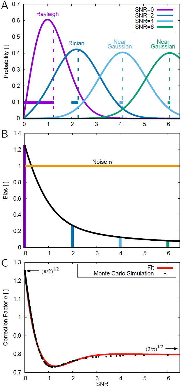
Single-shot diffusion-weighted MRI is plagued by noise. Noise not only makes viewing of fine details more difficult, but also introduces a bias that will result in erroneously lower ADCs and a more pronounced non-monoexponential diffusion signal decay. The resulting distribution of observed signals is known as Rician distribution (Fig. 1) [1]. Simple magnitude signal averaging will not eliminate the bias and complex signal averaging can be difficult, since it requires phase correction [2,3]. The signal bias can be corrected, provided expected signal <S> and Gaussian noise $$$\sigma_g$$$ can be determined [1,4], e.g., through averaging of repeated measurements and analysis of the Rayleigh distributed noise in an area of no signal. One potential problem with this approach is that $$$\sigma_g$$$ varies across the field of view. In this case an additional scan without RF excitation could be performed. Another problem is that many advanced reconstruction algorithms threshold out low signal areas. Overall, this approach involves additional time consuming measurements, which except for noise related variations do not really contribute any new information.Methods
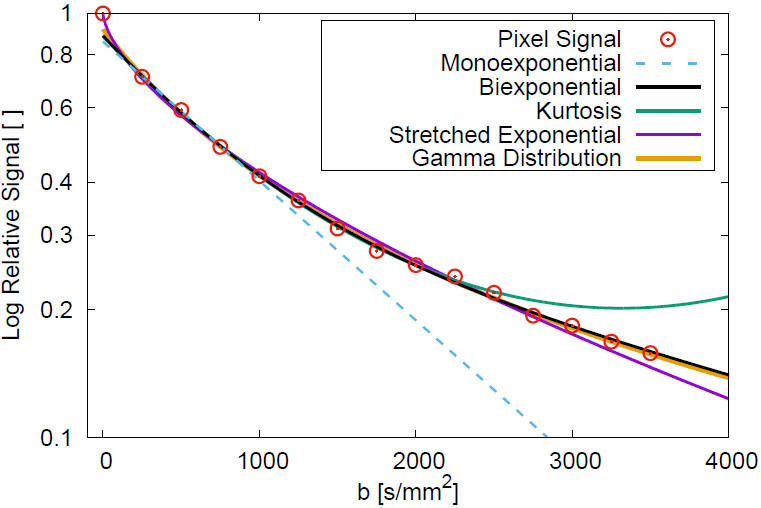
We propose a novel approach, where all measurements contribute meaningful information and at the same time allow the determination of <S> and $$$\sigma_g$$$ for each pixel position. We use the fact that model functions describe the signal decay well (Fig. 2) and that residual differences (at least up to a certain b-factor) can be considered predominantly noise related. Except for the kurtosis model with cumulant expansion, model fits are strictly monotonously decaying. Thus, there is no risk that with increasing number of parameters the residuals vanish.The fit conducted over N samples provides fitted signals $$$\hat{s}_i$$$ that are as good or even better estimates of the expected signal <$$$s_i$$$> than could be obtained with N averages (Fig. 3). The absolute residuals between fitted signals $$$\hat{s}_i$$$ and measured signals $$$s_i$$$, i.e., $$$r_i$$$ $$$=|\hat{s}_i-s_i$$$| are proportional to the SD of noise. Considering the distribution of $$$r_i$$$ at each b-factor, one can conjecture that the mean or expected $$$r_i$$$, i.e., <$$$r_i$$$> = $$$\alpha\cdot\sigma_g$$$,where $$$\alpha$$$ is a function of SNR. To find $$$\alpha$$$, we ran MonteCarlo simulations and fitted a function to the simulated data (Fig. 1C).
Now we resort to the realistic case of having a single realization of the diffusion signal decay. Again, assuming a perfect fit, an unbiased estimator of $$$\sigma_g$$$ at each b-factor would be $$$r_i/\alpha(\theta_i)$$$, where $$$\theta_i$$$ equals the SNR at $$$\hat{s}_i$$$.If we sum up all N estimations, we obtain a single unbiased estimator of $$$\sigma_g$$$:
\begin{equation}\sigma_g =\frac{1}{N}\sum_{i=1}^{N}r_i/\alpha(\theta_i)\end{equation}
At this point, we do not know any of the $$$\theta_i$$$ values. But as an initial guess, we can assume a Gaussian signal distribution for all $$$s_i$$$, where $$$r_i$$$ follows a half-folded normal distribution with $$$\alpha=\sqrt{2/\pi}$$$. We now have initial guesses of $$$\sigma_g$$$ and of N expected signals <$$$s_i$$$> at respective b-factors. For each <$$$s_i$$$> the Rician bias that would arise can then be calculated analytically. We subtract this bias value from our measured signal $$$s_i$$$ and finally obtain a bias corrected signal value $$$s_i^c$$$ to which we again can apply our model fit. This process is performed iteratively to obtain increasingly better estimates of $$$\sigma_g$$$ and of N $$$s_i^c$$$ values with associated bias. The standard deviation of the noise distribution varies with SNR from $$$\sigma_g$$$ when measured signals are Gaussian distributed to $$$\sqrt{(4-\pi)/2}\cdot\sigma_g$$$ when measured signals are Rayleigh and, therefore, much more narrowly distributed. The standard deviation of noise as a function of SNR can be determined analytically and can be accounted for by using different weights to each measurement. Multi-coil reconstruction can introduce signals that follow a non-central $$$\chi$$$ distribution [4,5]. With parallel imaging, which was used here, however, signals can be considered Rician distributed [6].
Results
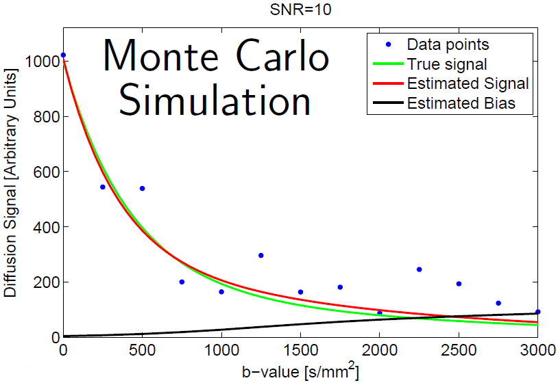
The process converges after a few iterations and the estimation of fit parameters is reliable, as long as SNR does not fall below 1 over an extended range of b-factors, e.g., with unsuitable experiment design. Bias correction results from Monte-Carlo simulations are presented in Fig. 4. The virtual averaging effect of a 21 b-factor protocol was estimated to be 4-fold at b0 and 16-fold at 3000 s/mm2. Results of bias correction of in vivo scans are presented in Fig. 5.
Discussion and Conclusion
The new approach for bias correction favors a multi-b protocol, which usually is helpful to reliably characterize a non-monoexponential decay. Together with the proposed algorithm signal averaging is achieved for all b-factors, noise is estimated and bias is corrected.Acknowledgements
ALFGBG-449801, CAN2017/558, NIH R01 CA160902
References
1) Gudbjartsson H and Patz S. The Rician distribution of noisy MRI data. Magn Reson Med, 34(6):910–4, 1995.
2) Prah DE, Paulson ES, Nencka AS, and Schmainda KM. A simple method for rectified noise floor suppression: Phase-corrected real data reconstruction with application to diffusion-weighted imaging. Magn Reson Med, 64(2):418–29, 2010.
3) Eichner C, Cauley SF, Cohen-Adad J, Moeller HE, Turner R, Setsompop K, and Wald LL. Real diffusion-weighted MRI enabling true signal averaging and increased diffusion contrast. NeuroImage,122:373–384, 2016.
4) Koay CG and Basser PJ. Analytically exact correction scheme for signal extraction from noisy magnitude MR signals. J Magn Reson, 179(2):317–22, 2006.
5) Constantinides CD, Atalar E, and McVeigh ER. Signal-to-noise measurements in magnitude images from NMR phased arrays. Magn Reson Med, 38(5):852–857, 2004.
6) Aja-Fernandez S, Vegas-Sanchez-Ferrero G, and Tristan-Vega A. Noise estimation in parallel MRI:GRAPPA and SENSE. Magn Reson Imaging, 32:281–290, 2014.
Figures
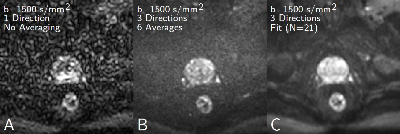
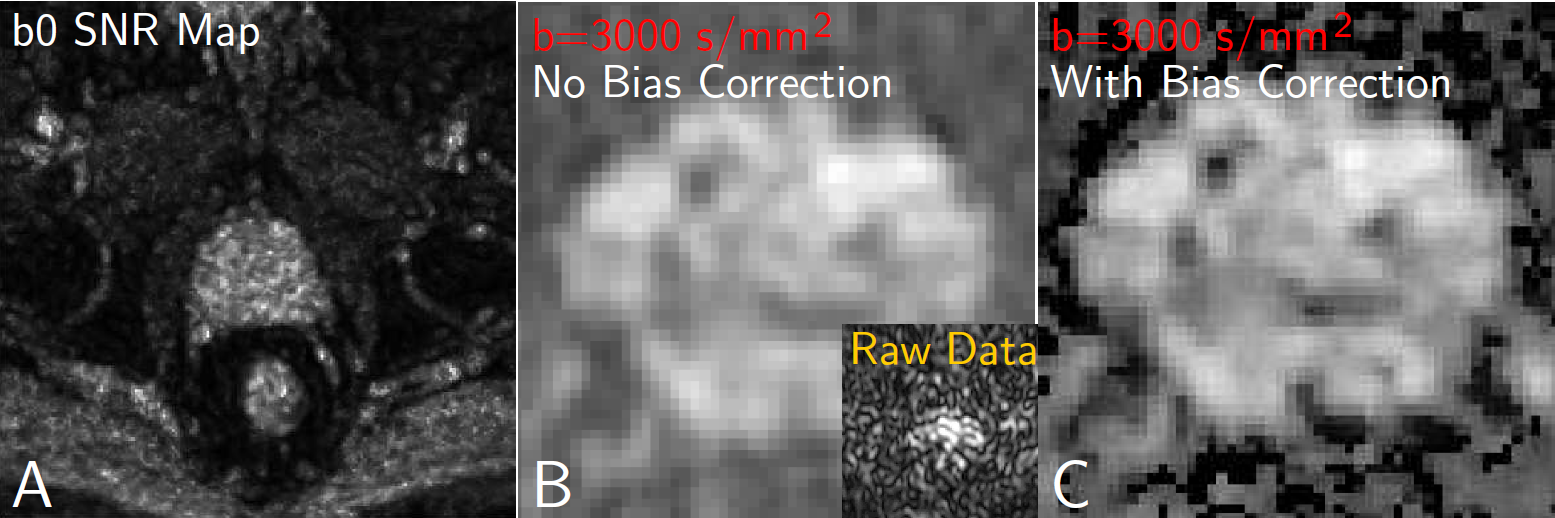
A) Estimated SNR map for the acquired and unaveraged b=0 image. The average SNR within the prostate measured with this map was 22. B) Detail of image synthesized from the complete set of data without signal bias correction for b=3000 s/mm2. The insert shows the original unaveraged raw data of a single diffusion encoding direction at b=3000 s/mm2. It emphasizes that at b=3000 s/mm2 and with external coil arrays useful data cannot be obtained unless excessive signal averaging is employed. C) Same area and b-factor as in B) but with signal bias correction applied. Within the prostate, contrast is clearly elevated.