3396
Correction of systematic errors in DTI imaging caused by gradient nonlinearity using gradient field maps measured by diffusion imaging of an isotropic diffusion phantom.1Quantitative Medical Imaging Section, National Institute of Biomedical Imaging and Bioengineering, NIH, Bethesda, MD, United States, 2Vanderbilt University Medical Center, Nashville, TN, United States
Synopsis
Gradient nonlinearity causes systematic errors in the measurement of DTI parameters. These errors can be greatly reduced if the actual fields generated by the gradient coils is known. Although the gradient field maps are known to the manufacturers, many users do not have access to them. We describe a method for measuring the gradient field maps using a set of diffusion weighted images of an isotropic diffusion PVP phantom. We use the field maps to analyze a DTI study of the phantom and compare the results to analysis performed without the field maps. The results show that the method works well.
Introduction
Nonlinearity in the magnetic field produced by gradient coils causes systematic errors in computed DTI parameters. If the actual field produced by each gradient coil as a function of position is known, these errors can be greatly reduced1. Since manufacturers typically will not give users the field gradient field maps without a research agreement, which many users lack, to correct the systematic errors users must measure the field maps themselves. The field maps can be measured by acquiring gradient echo images of an oil phantom with different setting of the linear shims and computing the fields from the change in phase2. We present an alternative method using diffusion imaging
of a homogenous
isotropic diffusion phantom containing Polyvinylpyrrolidone
(PVP) water solution3,4.
Theory
The signal Sq in voxel q of a diffusion weighted image of an isotropic diffusion phantom with is
(1) $$$S^q=S_0^q exp(-D\ tr(\bf b))$$$
where $$$S_0^q$$$ is the signal in voxel q without diffusion weighting, D is the diffusivity of the phantom, and tr(b) is the trace of the b-matrix.
For an ideal gradient set, the b-matrix is typically expressed as a dyad
(2) $$$b_{ij}=\kappa G_iG_j$$$
where κ is a constant that depends on the timing of the pulse sequence and Gi is the prescribed gradient sensitization in the i(=x,y,z)-direction. The effect of non-linear gradients can be taken into account by writing1
(3) $$$G_i={{\partial B^i}\over {r_j}}G^p_j$$$
where $$$G^p_j$$$ is the prescribed gradient, Bi is the field produced by gradient coil i (=x,y,z), and ri = x, y, or z for i=1, 2, or 3, respectively.
The field produced by the gradient coils is
(4) $$$B^i(r,\theta,\phi)=\sum_{l,m} \alpha_{lm}(c_{lm}^ir^lP_{lm}cos(\theta))cos(\phi)+s_{lm}^ir^lP_{lm}(cos(\theta))sin(\phi))$$$
where (r, θ, φ) are the spherical coordinates of an image point, Plm(x) is the associated Legendre polynomial, αlm is a normalization constant, and slm and clm are expansion coefficients. Manufacturers also use expansion (4) to describe the fields produced by the gradient coils, but a source of confusion and possible error is different values for the normalization constants.
To estimate the expansion coefficients, we acquire a set of diffusion weighted images and find the values of cilm and silm that minimizes χ2. In addition to the clm and slm, best fit values of diffusivity D and unattenuated signal S0 also have to be computed. Due to B0 inhomogeneity, S0 is a function of position, so it cannot be described by a single parameter. To reduce the number of parameters and thereby increase the stability of the fit, we divide the diffusion weighted images by the unattenuated reference image and fit the attenuation function
(5) $$$A={S\over S_0}$$$.
(6) $$$\chi^2=\sum_{q}(A^{qp}_{measured}-A^{qp}(c_{lm}^i,s_{lm}^i))^2 $$$
where the superscript q labels the voxel and the superscript p labels the image, and A is defined by Eqs 1-5, and $$$A^{qp}_{measured}$$$ is the normalized diffusion image p.
The problem of minimizing χ2 is not well defined because Eq 1 depends only on the product of the expansion coefficients and the diffusivity D. We therefore further assume that the gradients are properly calibrated and set the terms that describe the "ideal" gradient to 1.
The minimum number of images required to determine the expansion coefficients clm and slm for a single gradient is 2: an unweighted image and an image with diffusion weighting in the desired direction (x, y, or z only). In practice, the contribution of the imaging gradients to the diffusion weighting causes a systematic error in the derived fit parameters. To reduce the effect of the imaging gradients, we acquire a second image with the polarity of the diffusion pulses reversed. To compute expansion coefficients for all three gradients we therefore need 7 images.
Methods
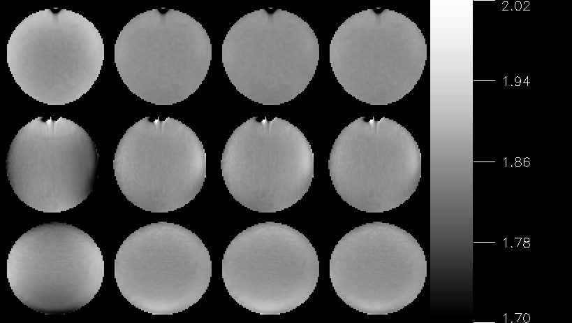
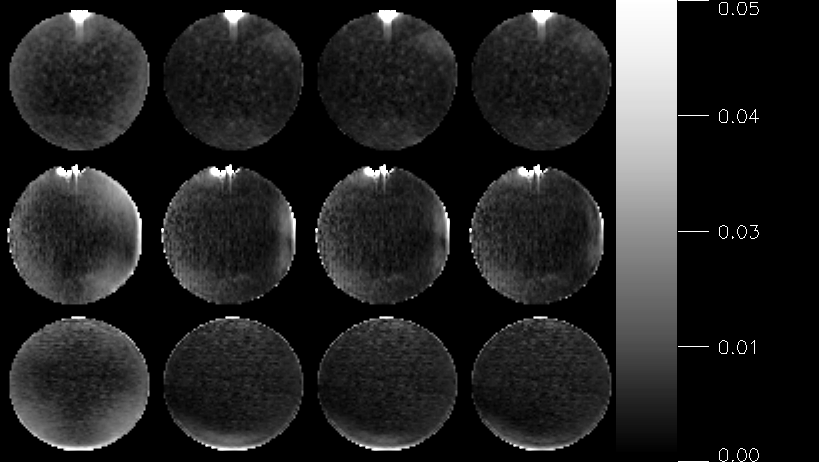
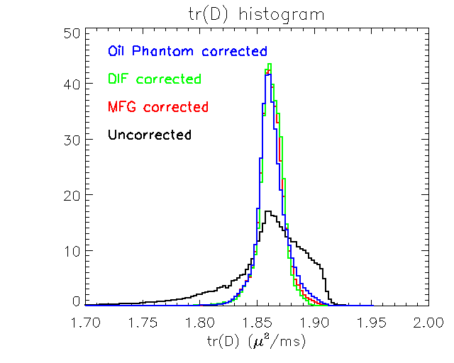
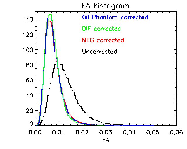
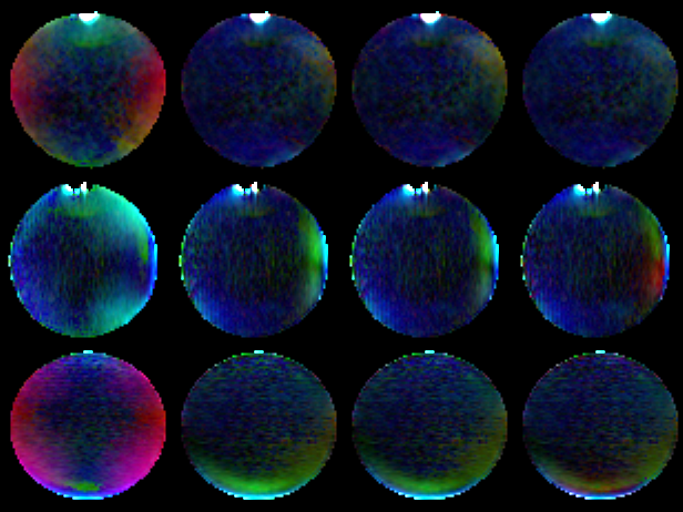
All images were acquired on a Philips Achieva 3T Scanner. We computed the expansion parameters from the minimum set (described above with b=1500) of 7 images of an isotropic diffusion PVP phantom. We also acquired a DTI data set comprising three shells of 32 directions each plus six unweighted images. All images used EPI readout and single echo sensitization. DTI parameters were computed 4 ways: 1) No correction, 2) Corrected with Diffusion DTI derived gradient field maps, 3) Corrected with GRE phase image derived field map2, and 4) Corrected with manufacturer supplied field map. Results are shown in the figures and described in the captions.Discussion and Conclusions
The correction greatly reduces the artifacts due to gradient inhomogeneity, and the proposed method produces tr(D) and FA maps almost indistinguishable from analysis using field maps obtained by other methods. Note that the method does not require an anisotropic diffusion phantom; only seven images of an isotropic diffusion phantom are needed. The proposed method can also improve the accuracy of diffusion metrics computed with other methods such as HARDI and NODDI.Acknowledgements
No acknowledgement found.References
1. Bammer R1, Markl M, Barnett A, Acar B, Alley MT, Pelc NJ, Glover GH, Moseley ME. Analysis and generalized correction of the effect of spatial gradient field distortions in diffusion-weighted imaging. Magn Reson Med. 2003 Sep;50(3):560-9.
2. Rogers BP, Blaber J, Newton AT, Hansen CB, Welch EB, Anderson AW, Luci JJ, Pierpaoli C, Landman BA. Phantom-based field maps for gradient nonlinearity correction in diffusion imaging. Proc SPIE Int Soc Opt Eng. 2018 Mar;10573. pii: 105733N. doi: 10.1117/12.2293786. PMID: 29887658; PMCID: PMC5990280.
3. Carlo Pierpaoli1, Joelle Sarlls1, Uri Nevo1,2, Peter J. Basser1, Ferenc Horkay1 Polyvinylpyrrolidone (PVP) Water Solutions as Isotropic Phantoms for Diffusion MRI Studies, ISMRM 2009, page: 1414
4. United States Patent 9,603,546 Horkay et al. Phantom for diffusion MRI imaging March 28, 2017
Figures