3394
Impact of processing options on histogram metrics extraction from DWI in cerebral small vessel disease1Department of Bioengineering, ISR-Lisboa/LARSyS, Instituto Superior Técnico - Universidade de Lisboa, Lisbon, Portugal, 2Neurology Department, Hospital Egas Moniz, Centro Hospitalar de Lisboa Ocidental, Lisbon, Portugal, 3CEDOC - Nova Medical School, New University of Lisbon, Lisbon, Portugal, 4Faculdade de Medicina, Universidade de Lisboa, Lisbon, Portugal, 5Imaging Department, Hospital da Luz, Lisbon, Portugal
Synopsis
Biomarkers based on diffusion-weighted imaging (DWI) have been proposed as potential disease biomarkers in several brain conditions including cerebral small vessel disease (SVD). Often histogram-based metrics are extracted, but findings across studies are somehow inconsistent. Here, we investigated the impact of several processing options for extracting histogram metrics of fractional anisotropy (FA) and mean diffusivity (MD) from DWI. We considered two white matter regions-of-interest with different interpolation and thresholding options, as well as different numbers of bins. We found that processing options significantly impacted histogram metrics, which in some cases significantly affects the ability to discriminate between patient and controls.
Introduction
Biomarkers based on diffusion-weighted imaging (DWI) have been proposed as potential disease biomarkers in several brain conditions including cerebral small vessel disease (SVD)1. Often histogram-based metrics are extracted, but findings across studies have been somehow inconsistent2–5. For example, Baykara et al. suggested using the mean diffusivity (MD) histogram peak width (extracted from the Tract-Based Spatial Statistics (TBSS)6 skeleton) as a predictor of processing speed (PS) impairment. In contrast, Lawrence et al. suggested the MD histogram peak height in a normal appearing white matter (NAWM) mask as the best PS predictor. Here, we aimed to investigate the impact of several processing options on DWI histogram metrics of MD and fraction anisotropy (FA), namely: the region-of-interest (TBSS vs. NAWM), the type of interpolation used in the registration between different imaging spaces, the threshold used for the TBSS skeleton, and the number of bins selected for the histogram.Methods
A sample of 17 SVD patients (50±9 yrs) and 12 healthy controls (HC) (52±6 yrs) was imaged on a 3T Siemens Verio scanner, including: (1) T1-weighetd MPRAGE (1mm isotropic); (2) T2-weighted FLAIR (0.7x0.7x3.3 mm3); (3) DWI-EPI (TR/TE=4800/107 ms, 25 contiguous slices, 1.7x1.7x5.2 mm3 with 3 repetitions of diffusion sensitizing gradients along 20 directions with b=0/1000 s/mm2). DWI images were pre-processed for eddy currents distortion corrections using FSL’s tools (fsl.fmrib.ox.ac.uk). Tensor fitting was performed to the DWI images with FSL’s dtifit, so as to obtain FA and MD maps.
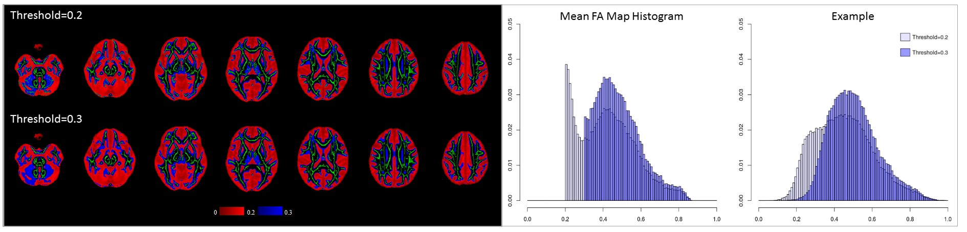
A white matter skeleton in standard MNI space7 was derived from the FA maps using TBSS. The non-linear registration of the TBSS mask to MNI space was tested using linear and nearest neighbour interpolation (ANTs tools, http://stnava.github.io/ANTs/). Also different FA values (0.2 and 0.3) were tested for skeleton thresholding (Fig. 1).
For the NAWM mask, we performed linear registration using FSL’s FLIRT to transform between DWI and MPRAGE spaces considering nearest neighbor and trilinear interpolation methods. White matter hyperintensities (WMH) were first manually segmented on the FLAIR images. The MPRAGE image was segmented into white matter (WM), gray matter and cerebrospinal fluid (CSF) using FSL’s FAST8. To define the mask of NAWM, FLAIR images were affinely registered to the MPRAGE and the transformation applied to the WMH mask, which was then subtracted from the total WM mask.
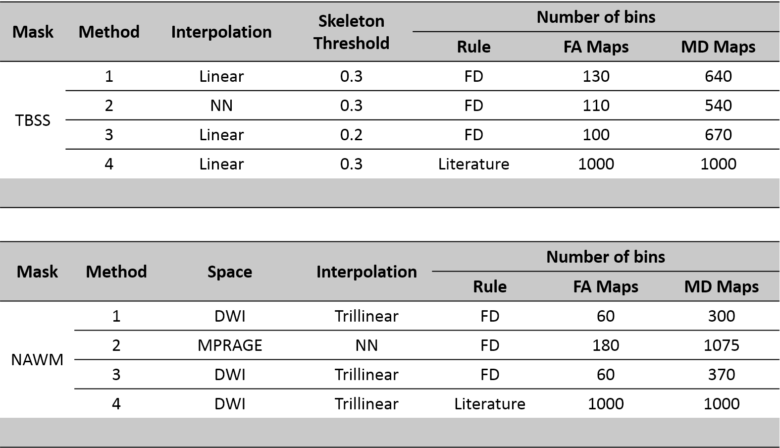
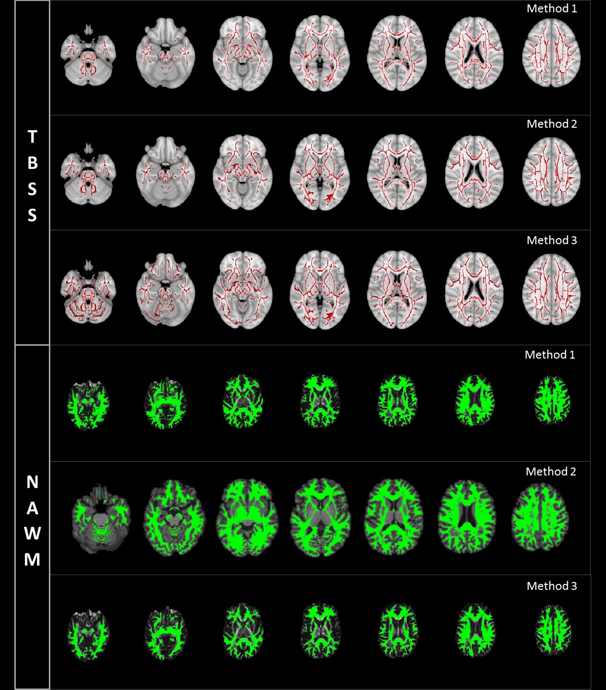
For each mask (TBSS and NAWM), the optimal number of bins for computing the histograms was computed using the Freedman-Diaconis rule; for comparison we also tested 1000 bins as this is frequently used in the literature. The 4 different methods used to obtain the histograms in the TBSS and NAWM masks are summarised in Fig.2. Illustrative examples of the 3 first processing methods evaluated are shown in Fig.3.
Histogram analyses of both FA and MD maps were performed using R (https://www.r-project.org/). The histogram metrics median, peak height, peak value and peak width were extracted. To investigate the effects of the methods, a two-way repeated measures ANOVA was performed on each metric using method as a fixed within-subject effect and group as a random between-subjects effect. When the interaction between factors was significant (p<0.05), we performed independent samples T-tests.
Results
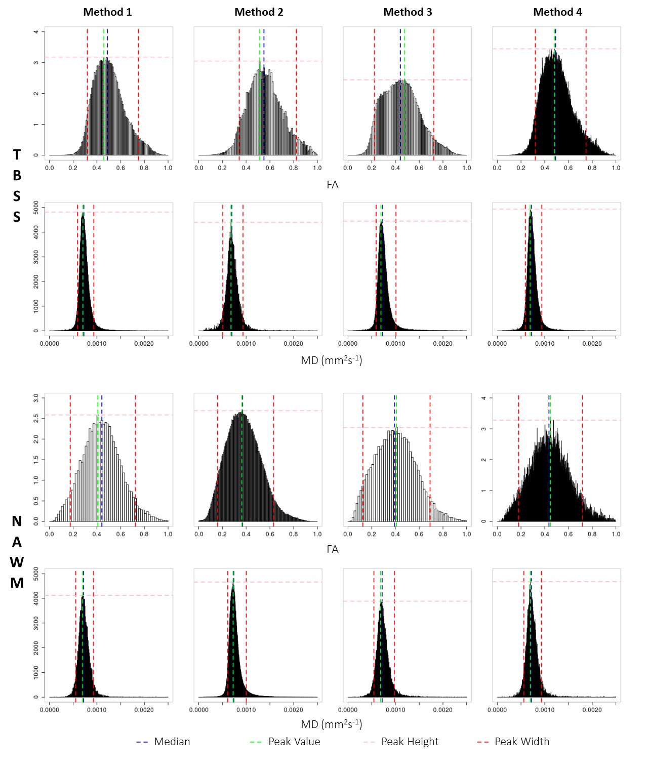
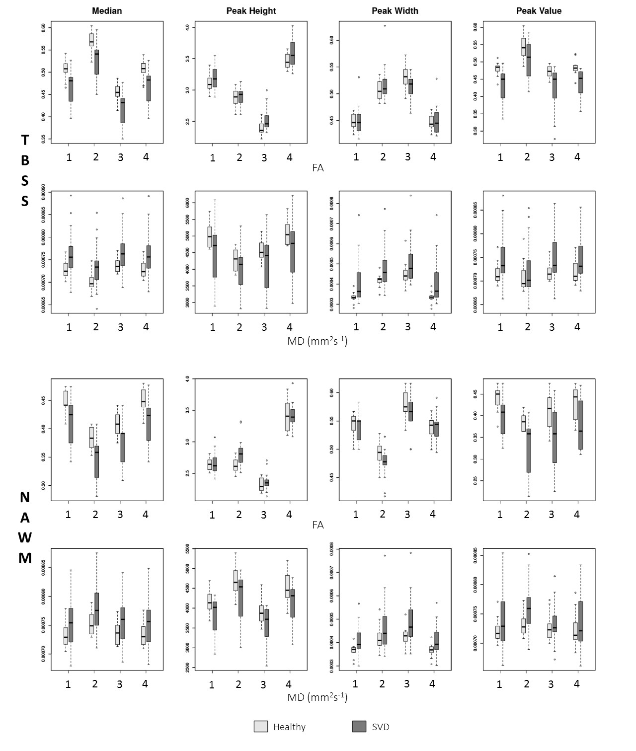
Boxplots showing the distributions across healthy controls and SVD patients of FA and MD histogram metrics, obtained using each method tested for each considered mask, are shown in Fig.5. Statistical analysis showed significant mains effects of method for all metrics. Moreover, significant interactions were also found between method and group for the following metrics: (1) TBSS FA: median (p=0.02), peak height (p=0.04) and peak width (p<0.001); (2) TBSS MD and NAWM FA: peak height (p=0.04;p<0.01) and peak width (p=0.03;p<0.001). In fact, both methods 1 and 4 enabled to differentiate between groups using FA median, MD peak height and MD peak width with the TBSS mask. Interestingly, the peak value never showed significant interactions.Conclusions
Our results show that the processing options made to generate the histograms have significant impact on the values of FA and MD histogram metrics extracted from DWI, which in some cases significantly affects the ability to discriminate between patient and controls. Methods 1 and 4 (with two different numbers of bins) show the best potential for differentiating between groups, while different interpolations or thresholding options might compromise such discriminative power. Overall, our results highlight the need to carefully select the processing method when extracting histogram metrics of DWI parameters.Acknowledgements
This work was funded by FCT grants PTDC/BBB-IMG/2137/2012 and UID/EEA/50009/2013.References
1. Banerjee G, Wilson D, Jäger HR, Werring DJ. Novel imaging techniques in cerebral small vessel diseases and vascular cognitive impairment. Biochim Biophys Acta - Mol Basis Dis. 2015;1862(5):926-938. doi:10.1016/j.bbadis.2015.12.010.
2. Croall ID, Lohner V, Moynihan B, et al. Using DTI to assess white matter microstructure in cerebral small vessel disease ( SVD ) in multicentre studies. Clin Sci. 2017;131:1361-1373. doi:10.1042/CS20170146.
3. Zeestraten EA, Lawrence AJ, Lambert C, et al. Change in multimodal MRI markers predicts dementia risk in cerebral small vessel disease. Neurology. 2017:10--1212. doi:10.1212/WNL.0000000000004594.
4. Baykara E, Gesierich B, Adam R, et al. A Novel Imaging Marker for Small Vessel Disease Based on Skeletonization of White Matter Tracts and Diffusion Histograms. Ann Neurol. 2016;80(4):581-592.
5. Lawrence AJ, Patel B, Morris RG, et al. Mechanisms of Cognitive Impairment in Cerebral Small Vessel Disease: Multimodal MRI Results from the St George ’ s Cognition and Neuroimaging in Stroke (SCANS) Study. 2013;8(4). doi:10.1371/journal.pone.0061014.
6. Smith SM, Jenkinson M, Johansen-Berg H, et al. Tract-based spatial statistics: Voxelwise analysis of multi-subject diffusion data. Neuroimage. 2006;31(4):1487-1505. doi:10.1016/j.neuroimage.2006.02.024.
7. Grabner G, Janke AL, Budge MM, et al. Symmetric atlasing and model based segmentation: an application to the hippocampus in older adults. In: Med Image Comput Comput Assist Interv Int Conf Med Image Comput Comput Assist Interv. ; 2006:58–66. doi:http://dx.doi.org/10.1007/11866763_8.
8. Zhang Y, Brady M, Smith S. Segmentation of brain MR images through a hidden Markov random field model and the expectation-maximization algorithm. IEEE Trans Med Imag. 2001;20(1):45-57.
Figures