3367

A novel connectomics metric for investigating the structural-functional relationship in the brain

Oren Civier^1,2, Marion Sourty^1,2, and Fernando Calamante^1,2,3,4

¹School of Aerospace, Mechanical and Mechatronic Engineering, The University of Sydney, Sydney, Australia, ²Brain and Mind Centre, The University of Sydney, Sydney, Australia, ³Sydney Imaging, The University of Sydney, Sydney, Australia, ⁴Florey Department of Neuroscience and Mental Health, University of Melbourne, Melbourne, Australia

Synopsis

We present a novel connectomics metric that quantifies the relationship between structural connectivity (SC) and functional connectivity (FC) in each connection in the brain. The metric is based on a biologically meaningful and quantitative measure of SC, followed by normalization of both modalities to a common scale. We demonstrated the utility of the metric in examining structural-functional relationships in pairs of homologous connections, detecting homologues that are dissimilar. The metric is more informative than using FC in isolation, and might provide insights into factors that contribute to FC beyond the strength of SC (e.g., indirect connections, organization of fibres).

Introduction

Past studies showed that structural connectivity (SC, the strength of the direct connection between two nodes in a connectome based on tractography) broadly predicts functional connectivity (FC, defined here as the correlation between pair of nodes based on resting-state fMRI).^1-5 However, the development of methods to exploit this has been limited. Here we define a novel connectomics metric that quantifies the relationship between SC and FC, and demonstrate its use for comparing the left-hemisphere and right-hemisphere connections in each pair of homologous connections (or homologous pair). Studying the similarity between corresponding left and right connections is important because it may indicate, for example, on their ability to compensate for each other.

Our metric relies on two recent advances:

1. Quantitative measure of SC that are more biologically meaningful.⁶ We use SIFT2.⁷

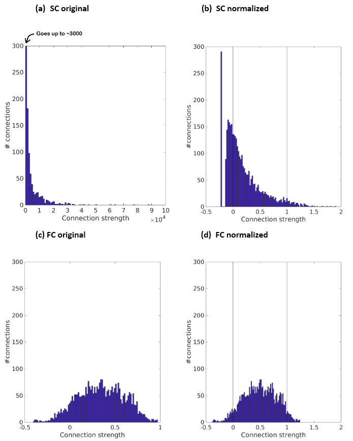
2. Findings that the (within-brain) distribution of SC (e.g., relatively few connections are several orders of magnitude stronger than most other connections)^8,9 is very different from that of FC (approximately normal distribution).¹⁰ We apply a transformation to make the distributions more similar.

Methods

Our metric is defined as the function $$f^{SC\rightarrow{FC}}_{i,j,H}=N(FC_{i,j,H})-N(\sqrt[4]{SC_{i,j,H}})$$ $$$i\neq{j}$$$ are two brain regions in the same hemisphere, and $$$H$$$ indicates the (left or right) hemisphere. In a sense, the metric can be understood as the quantity that should be added to the normalized SC to get the normalized FC. Power of 1/4 was empirically chosen to eliminate the long/heavy right tail of SC distribution, while still giving strong connections a considerable advantage. We did not alter the leftward skewness (cf.¹) because there should indeed be more connections with weak SC than with weak FC (FC but not SC may increase due to indirect connections). See Fig. 1 for the definition of $$$N(x)$$$.

We included 50 pre-processed datasets from the Human Connectome Project (HCP).^11-14

Diffusion MRI: Bias-field correction¹⁵ and multi-shell multi-tissue CSD¹⁶ to estimate fibre orientation distributions. 10 million probabilistic streamlines using iFOD2¹⁷ and ACT¹⁸. Weight for each streamline using SIFT2.⁷ SC connectome using 84 regions⁶ (cortex and cerebellum, FreeSurfer¹⁹; subcortical regions, FSL-FIRST²⁰); connection strengths are sums of relevant streamlines’ weights. Processing was performed using MRtrix3 (www.mrtrix.org)²¹.

Resting-state fMRI: FC computed from Pearson correlation between each pair of regional mean time-courses (same 84 parcellated regions). We did not discard negative connections as their contribution was negligible in our specific analysis.

For each subject, we calculated $$$f^{SC\rightarrow{FC}}_{i,j,H}$$$ for every connection in the graph.

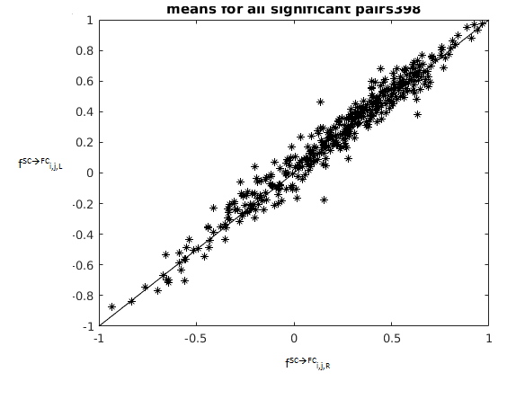
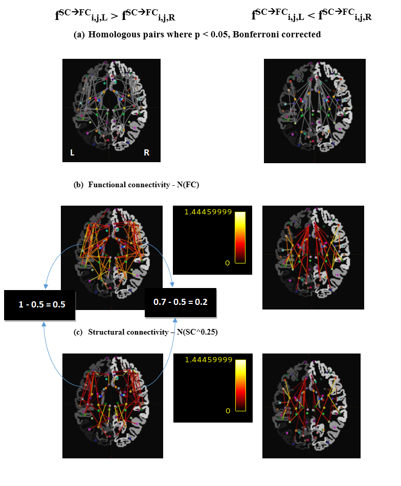
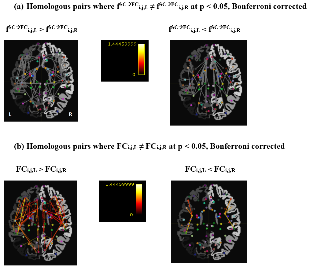
To illustrate the method, we identified homologous pairs where $$$f^{SC\rightarrow{FC}}_{i,j,L}$$$ and $$$f^{SC\rightarrow{FC}}_{i,j,R}$$$ correlate (using Pearson’s r, 50 subjects), and then detected the pairs where $$$f^{SC\rightarrow{FC}}_{i,j,L}$$$ and $$$f^{SC\rightarrow{FC}}_{i,j,R}$$$ are significantly different (using paired t-test, same 50 subjects). For both analyses, we used Bonferroni correction to account for the 861 tests conducted (one for each homologous pair). We also repeated the analysis using $$$FC_{i,j,H}$$$ rather than $$$f^{SC\rightarrow{FC}}_{i,j,H}$$$ to specifically examine homologous pairs where FC is lateralized.

Results

Fig. 2 shows all homologous pairs where $$$f^{SC\rightarrow{FC}}_{i,j,L}$$$ and $$$f^{SC\rightarrow{FC}}_{i,j,R}$$$ are systematically related. In these pairs there is a good agreement between metric value on the left and right, with a few exceptions. These exceptions are explored in more detail in Fig. 3, which shows homologous pairs where $$$f^{SC\rightarrow{FC}}_{i,j,L}$$$ and $$$f^{SC\rightarrow{FC}}_{i,j,R}$$$ are significantly different. Fig. 4 shows the homologous pairs where FC is significantly lateralized, and highlights (thick lines) those pairs where the lateralization cannot be explained by the underlying SC.

Discussion

The introduced metric could capture the broadly similar structural-functional relationship in the left and right connections of each homologous pair (Fig. 2). Even when FC was different between left and right homologues, SC often expressed a similar difference, keeping the metric value comparable across the two hemispheres (Fig. 4, thin lines). Importantly, the metric was sensitive enough to detect homologous pairs where the structural-functional relationship differed across hemispheres (Fig. 3). This might indicate, for example, that in these particular homologous pairs, each homologue might have a somewhat different fibre wiring (not in strength, but in organization), and that this induces the different relationship with FC. Because of the different wiring bilaterally, we speculate that contralateral compensation after lesion might be unlikely for these particular pairs. Alternatively, the difference might relate to the differential contribution from indirect SC.^1,4,5

Conclusion

We proposed a connectomics structural-functional metric that may have many possible applications. For example, the detection of homologous connections with different structural-functional relationship in the left and right homologues (demonstrated here), or the detection of functional plasticity (in a single connection) that is not accompanied by corresponding structural plasticity in the same particular connection (thus, remote structural plasticity affecting indirect connectivity might have contributed).

Acknowledgements

This research was supported by the National Health and Medical Research Council of Australia, the Australian Research Council, and Melbourne Bioinformatics at the University of Melbourne, grant number UOM0048. Data were provided by the Human Connectome Project, WU-Minn Consortium (Principal Investigators: David Van Essen and Kamil Ugurbil; 1U54MH091657) funded by the 16 NIH Institutes and Centers that support the NIH Blueprint for Neuroscience Research; and by the McDonnell Center for Systems Neuroscience at Washington University. We also thank Xiaoyun Liang and Chun-Hung Yeh for their assistance.

References

1. Honey CJ, Sporns O, Cammoun L, Gigandet X, Thiran JP, Meuli R, et al. Predicting human resting-state functional connectivity from structural connectivity. Proc Natl Acad Sci U S A. 2009;106(6):2035-40.

2. Goñi J, van den Heuvel MP, Avena-Koenigsberger A, de Mendizabal NV, Betzel RF, Griffa A, et al. Resting-brain functional connectivity predicted by analytic measures of network communication. Proceedings of the National Academy of Sciences. 2014;111(2):833-8.

3. Rosenthal G, Vasa F, Griffa A, Hagmann P, Amico E, Goni J, et al. Mapping higher-order relations between brain structure and function with embedded vector representations of connectomes. Nat Commun. 2018;9(1):2178.

4. Horn A, Ostwald D, Reisert M, Blankenburg F. The structural–functional connectome and the default mode network of the human brain. Neuroimage. 2014;102:142-51.

5. Skudlarski P, Jagannathan K, Calhoun VD, Hampson M, Skudlarska BA, Pearlson G. Measuring brain connectivity: diffusion tensor imaging validates resting state temporal correlations. Neuroimage. 2008;43(3):554-61.

6. Smith RE, Tournier J-D, Calamante F, Connelly A. The effects of SIFT on the reproducibility and biological accuracy of the structural connectome. Neuroimage. 2015;104:253-65.

7. Smith RE, Tournier J-D, Calamante F, Connelly A. SIFT2: Enabling dense quantitative assessment of brain white matter connectivity using streamlines tractography. Neuroimage. 2015;119:338-51.

8. Ercsey-Ravasz M, Markov NT, Lamy C, Van Essen DC, Knoblauch K, Toroczkai Z, et al. A predictive network model of cerebral cortical connectivity based on a distance rule. Neuron. 2013;80(1):184-97.

9. Oh SW, Harris JA, Ng L, Winslow B, Cain N, Mihalas S, et al. A mesoscale connectome of the mouse brain. Nature. 2014;508(7495):207.

10. Fornito A, Zalesky A, Pantelis C, Bullmore ET. Schizophrenia, neuroimaging and connectomics. Neuroimage. 2012;62(4):2296-314.

11. Van Essen DC, Smith SM, Barch DM, Behrens TE, Yacoub E, Ugurbil K, et al. The WU-Minn human connectome project: an overview. Neuroimage. 2013;80:62-79.

12. Smith SM, Beckmann CF, Andersson J, Auerbach EJ, Bijsterbosch J, Douaud G, et al. Resting-state fMRI in the human connectome project. Neuroimage. 2013;80:144-68.

13. Glasser MF, Sotiropoulos SN, Wilson JA, Coalson TS, Fischl B, Andersson JL, et al. The minimal preprocessing pipelines for the Human Connectome Project. Neuroimage. 2013;80:105-24.

14. Van Essen DC, Ugurbil K, Auerbach E, Barch D, Behrens T, Bucholz R, et al. The Human Connectome Project: a data acquisition perspective. Neuroimage. 2012;62(4):2222-31.

15. Tustison NJ, Avants BB, Cook PA, Zheng Y, Egan A, Yushkevich PA, et al. N4ITK: improved N3 bias correction. IEEE transactions on medical imaging. 2010;29(6):1310-20.

16. Jeurissen B, Tournier J-D, Dhollander T, Connelly A, Sijbers J. Multi-tissue constrained spherical deconvolution for improved analysis of multi-shell diffusion MRI data. NeuroImage. 2014;103:411-26.

17. Tournier JD, Calamante F, Connelly A, editors. Improved probabilistic streamlines tractography by 2nd order integration over fibre orientation distributions. Proceedings of the international society for magnetic resonance in medicine; 2010.

18. Smith RE, Tournier J-D, Calamante F, Connelly A. Anatomically-constrained tractography: improved diffusion MRI streamlines tractography through effective use of anatomical information. Neuroimage. 2012;62(3):1924-38.

19. Desikan RS, Segonne F, Fischl B, Quinn BT, Dickerson BC, Blacker D, et al. An automated labeling system for subdividing the human cerebral cortex on MRI scans into gyral based regions of interest. Neuroimage. 2006;31(3):968-80.

20. Patenaude B, Smith SM, Kennedy DN, Jenkinson M. A Bayesian model of shape and appearance for subcortical brain segmentation. Neuroimage. 2011;56(3):907-22.

21. Tournier JD, Calamante F, Connelly A. MRtrix: diffusion tractography in crossing fiber regions. International Journal of Imaging Systems and Technology. 2012;22(1):53-66.

Figures

Fig . 1 Distributions before and after normalizations (a) Original $$$ SC$$$ (b) $$$N(\sqrt[4]{SC})$$$. To reduce the influence of possible outliers, $$$N(x)$$$ is a linear function that transforms the 5th and the 95th percentiles of the distribution of $$$x$$$ to 0 and 1, respectively. To reduce the influence of presumed spurious structural connections ($$$SC < 10$$$), percentile 0th of the $$$SC$$$ distribution was artificially set at 10. Accordingly, >5% of the values of $$$N(\sqrt[4]{SC})$$$ are smaller than 0. This procedure contributed to the metric having higher sensitivity in the range where connections are more likely real. (c) Original $$$FC$$$ (d) $$$N(FC)$$$.

Fig. 2 Group-average $$$f^{SC\rightarrow{FC}}_{i,j,L}$$$ against group-average $$$f^{SC\rightarrow{FC}}_{i,j,R}$$$. A data point on the diagonal (black line) indicates $$$f^{SC\rightarrow{FC}}_{i,j,L} = f^{SC\rightarrow{FC}}_{i,j,R}$$$. A data point above the diagonal indicates that the quantity that should be added to $$$ N(\sqrt[4]{SC})$$$ to get $$$N(FC)$$$ on the left hemisphere is greater than the quantity needed on the right hemisphere. A data point below the diagonal indicates that a greater quantity is needed on the right hemisphere. Importantly, for many of the data points on the diagonal, SC and FC are actually not the same across hemispheres; rather, only the relationship between SC and FC is the same

Fig. 3 Homologous pairs where $$$f^{SC\rightarrow{FC}}_{i,j,L} \neq f^{SC\rightarrow{FC}}_{i,j,R}$$$. (a) The homologous pairs were the difference is significant. (b) The average N(FC) for the connections from panel a. Hotter colours indicate higher values. (c) Average N(SC^0.25). Left column: $$$f^{SC\rightarrow{FC}}_{i,j,L} > f^{SC\rightarrow{FC}}_{i,j,R}$$$, indicating that these homologous pairs are plotted above the diagonal in Fig. 2. Right column: $$$f^{SC\rightarrow{FC}}_{i,j,L} < f^{SC\rightarrow{FC}}_{i,j,R}$$$, indicating that the pairs are plotted below the diagonal. For ease of interpretation, we only present differences driven by functional connectivity. Homologous nodes are represented by identically coloured circles. Blue arrows give an example for a specific pair of homologous connections.

Fig. 4 Homologous pairs where FC is significantly lateralized, and the lateralization cannot be explained by underlying SC. (a) As in Fig. 3. (b) Only shown are homologous pairs where $$$N(FC_{i,j,L}) ≠ N(FC_{i,j,R})$$$ Brighter colours for stronger connections. Homologous pairs where the relationship between $$$SC$$$ and $$$FC$$$ is different in the left and right hemispheres (pair also exists in panel a) are marked by thick lines. In these pairs, the lateralization of $$$FC$$$ is less likely due to lateralization of $$$SC$$$, and is possibly due to other factors (see Discussion). Other conventions as in Fig. 3.

Proc. Intl. Soc. Mag. Reson. Med. 27 (2019)

3367