3202
4D Real-time BOLD MRI in Genetically Engineered Mouse Brains with Acute Hypoxia ChallengeAnthony G Christodoulou1, George C Gabriel2, Cecilia W Lo2, and Yijen L Wu2,3
1Biomedical Imaging Research Institute, Cedars-Sinai Medical Center, Los Angeles, CA, United States, 2Developmental Biology, University of Pittsburgh, Pittsburgh, PA, United States, 3Rangos Research Center Animal Imaging Core, Children's Hospital of Pittsburgh of UPMC, Pittsburgh, PA, United States
Synopsis
The objective of this study is to develop 4D time-resolved high-resolution BOLD MRI by combining low-rank sparse imaging and compressed sensing. By expressing a dynamic BOLD image as the product of a set of basis images and temporal functions, we are able to capture differential dynamic BOLD responses to oscillating hypoxia challenge in high-resolution 3D space in genetically engineered mouse brains.
Introduction
Blood oxygenation level dependent (BOLD) contrast in conjunction with neuro-vascular coupling during neuronal activation has been used to map neuronal activities during cognitive tasks. To capture the fast temporal signal changes due to changes in deoxy-hemoglobin, BOLD MRI is usually acquired with low spatial resolution then super-imposed on high-resolution static anatomical images. However, this conventional approach can suffer from drawbacks like mis-match of the BOLD signal and the actual neuronal location; and low-resolution BOLD MRI can miss smaller loci of abnormal activities. The goal of this study is to establish 4D time-resolved BOLD MRI with both high-spatial and high-temporal resolution in the same scan.Methods
Our method uses a hybrid1 low-rank2 and sparse3 model to measure a dynamic BOLD image $$$\rho(\mathbf{r},t)$$$ (for spatial position $$$\mathbf{r}$$$ and time $$$t$$$) from undersampled $$$(\mathbf{k},t)$$$-space data. The low-rank model expresses the image as the outer product of a set of $$$L$$$ basis images $$$\{\psi_\ell(\mathbf{r})\}_{\ell=1}^L$$$ and $$$L$$$ temporal functions $$$\{\varphi_\ell(t)\}_{\ell=1}^L$$$:$$\rho(\mathbf{r},t)=\sum_{\ell=1}^L\psi_\ell(\mathbf{r})\varphi_\ell(t),$$ or in matrix form, $$$\mathbf{X=\Psi\Phi}$$$, where $$$X_{ij}=\rho(\mathbf{r}_i,t_j)$$$, $$$\mathit{\Psi}_{ij}=\psi_j(\mathbf{r}_i)$$$, and $$$\mathit{\Phi}_{ij}=\varphi_i(t_j)$$$. The sparse model expresses $$$\rho(\mathbf{r},t)$$$ as sparse in some transform domain, which we choose as the wavelet-spectral domain (i.e., that $$$\mathcal{F}_t\{\mathcal{W}_\mathbf{r}\{\rho(\mathbf{r},t)\}\}$$$ is sparse, where $$$\mathcal{W}_\mathbf{r}$$$ performs a spatial wavelet transform and $$$\mathcal{F}_t$$$ performs the temporal Fourier transform). This approach exploits the correlation of BOLD images over time as well as the transform sparsity of the image series to allow imaging with high spatiotemporal resolution. Data are acquired by alternating between collection of two sets of data: D1, which contains auxiliary “navigator” data collected at a high temporal sampling rate but a limited number of k-space trajectories, and D2, which contains sparsely sampled $$$(\mathbf{k},t)$$$ -space data with extended k-space coverage. This strategy capitalizes on the partially separated model’s decoupled resolution requirements: the high-speed data in D1 inform the temporal basis functions (i.e., the $$$\varphi$$$’s), and the full k-space data in D2 inform the spatial coefficient maps (i.e., the $$$\psi$$$’s), resulting in images with the high temporal resolution of D1 and the high spatial resolution of D2. This strategy allows a two-step image reconstruction process wherein temporal basis functions $$$\{\varphi_\ell(t)\}_{\ell=1}^L$$$ are determined from the singular value decomposition (SVD) of D1, and the spatial coefficient maps $$$\{\psi_\ell(\mathbf{r})\}_{\ell=1}^L$$$ are determined by fitting $$$\{\varphi_\ell(t)\}_{\ell=1}^L$$$ to D2 with sparse regularization. This final fitting step is performed according to$$\mathbf{\Psi}=\arg\min_\mathbf{\Psi}\|\mathbf{d}-E(\mathbf{\Psi\Phi})\|_2^2+\lambda\|\mathbf{W\Psi\Phi{F}}\|_1,$$where $$$\mathbf{d}$$$ are the data from D2, $$$E$$$ is the encoding operator comprising spatial encoding and undersampling, $$$\mathbf{W}$$$ is a spatial wavelet transform, and $$$\mathbf{F}$$$ is the temporal Fourier transform.Results
Figure 1 shows an example of real-time 4D BOLD MRI of a control wild-type (WT) mouse with 156-micron isotropic resolution with oscillating hypoxia challenge every 3 min. By separating the dynamic image into basis images and temporal functions, we are able to acquire high-resolution 4D images at the same time to capture the fast temporal BOLD signal changes responding to oscillating hypoxia challenges. The temporal BOLD signal profile from each voxel can be measured to allow sensitive detection of any voxel that displays hypoxia responses deviating from normal healthy brain tissue. Importantly, only the brain displayed BOLD signal changes upon oscillating hypoxia challenge whereas the head muscle showed little dynamic BOLD signal changes (Fig. 1). Figure 2 shows 4D BOLD MRI of a WT control mouse (Fig.2,A,D,G,J), a homozygous pcdha9 mutant mouse (Fig.2,B,E,H,K) and a Emx1-cre Sap130 f/ko mouse (Fig.2,C,F,I,L). Pcdha9 gene encodes protocadherinA9 mediating cell-cell adhesion, responsible for synaptic path finding. Sap130 encodes Sin3A-associated protein 130, a member of the histone deacetylase (HDAC) complex mediating chromatin repression. Emx1 is a mouse homologue of the Drosophila homeobox gene empty spiracles and its expression is restricted to the forebrain and hippocampus. Emx1-cre drives Sap130 deletion specifically restricted to the forebrain regions where Emx1 is expressed. Both mutant mice exhibited similar gross brain morphology (Fig.2 B,C) comparable to WT control (Fig.2A). However, the 4D MRI showed markedly different response patterns in responding to oscillating hypoxia challenge (Fig.2 D-F). WT (Fig.2D) showed good BOLD responses throughout the whole brain, except CSF and middle cerebral artery (MCA). Pcdha9 mutant brain (Fig2E) displayed decreased BOLD responses in the periventricular areas and hippocampus. Emx1-cre Sap-130 f/ko brain (Fig.2F) exhibited differential BOLD responses in the forebrain, mid-brain, and hindbrain regions. Temporal BOLD signal responses to the oscillating hypoxia challenge in selected regions (R1, R2, R3) are displayed as magnitude (Fig.2, G-I) and phase (Fig.2 J-L).Conclusion
Our 4D time-resolved BOLD MRI can capture the dynamic BOLD signals with high spatial and temporal resolution.Acknowledgements
The authors thank Nathan Salamacha, Cassandra Slover, Samuel Wyman, Lauren Myers, and Cullen Yang, for assisting with animals.References
1. Zhao B et al. IEEE-TMI 2012.
2. Liang Z-P. IEEE-ISBI 2007.
3. Lustig M et al. MRM 2007.
Figures
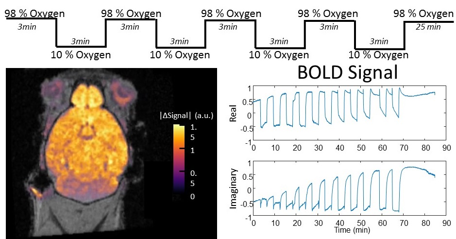
4D real-time BOLD MRI with
156-micron isotropic resolution of a wild-type (WT) control mouse acquired at
7-Tesla with TE=6ms. The oscillating hypoxia challenge with 10% oxygen was
imposed every 3 minutes during the 4D acquisition. The color scale shows
percent changes of the BOLD signals. The
pixels with signal changes upon oscillating hypoxia challenges are mainly
localized in the brain. The head muscle
signal did not change significantly between the high and low oxygen
states.

4D real-time BOLD MRI of a WT control mouse (A, D, G, J), a homozygous
pcdha9 mutant mouse (B, E, H, K) and a Emx1-cre driven flux Sap130 knockout
mouse with Sap130 specifically knocked out in the forebrain area (C, F, I,
L). (A-C) T2-weighted anatomical MRI
(D-F) BOLD response maps generated by the differences between the high and low
oxygen states. The color scales are
normalized to 300% of the averaged head muscle responses. (G-I) Magnitudes of
the dynamic BOLD responses in regions R1, R2, R3 depicted D-F. (J-L) phases of
dynamic BOLD responses of the regions.